The Full Stack 7-Steps MLOps Framework

A Framework for Building a Production-Ready Feature Engineering Pipeline

Lesson 1: Batch Serving. Feature Stores. Feature Engineering Pipelines.

This tutorial represents lesson 1 out of a 7-lesson course that will walk you step-by-step through how to design, implement, and deploy an ML system using MLOps good practices. During the course, you will build a production-ready model to forecast energy consumption levels for the next 24 hours across multiple consumer types from Denmark.

By the end of this course, you will understand all the fundamentals of designing, coding and deploying an ML system using a batch-serving architecture.

This course targets mid/advanced machine learning engineers who want to level up their skills by building their own end-to-end projects.

Nowadays, certificates are everywhere. Building advanced end-to-end projects that you can later show off is the best way to get recognition as a professional engineer.

Table of Contents:

• Course Introduction
• Course Lessons
• Data Source
• Lesson 1: Batch Serving. Feature Stores. Feature Engineering Pipelines.
• Lesson 1: Code
• Conclusion
• References

Introduction

At the end of this 7 lessons course, you will know how to:

• design a batch-serving architecture
• use Hopsworks as a feature store
• design a feature engineering pipeline that reads data from an API
• build a training pipeline with hyper-parameter tunning
• use W&B as an ML Platform to track your experiments, models, and metadata
• implement a batch prediction pipeline
• use Poetry to build your own Python packages
• deploy your own private PyPi server
• orchestrate everything with Airflow
• use the predictions to code a web app using FastAPI and Streamlit
• use Docker to containerize your code
• use Great Expectations to ensure data validation and integrity
• monitor the performance of the predictions over time
• deploy everything to GCP
• build a CI/CD pipeline using GitHub Actions

If that sounds like a lot, don't worry, after you will cover this course you will understand everything I said before. Most importantly, you will know WHY I used all these tools and how they work together as a system.

If you want to get the most out of this course, I suggest you access the GitHub repository containing all the lessons' code. I designed the articles so you can read and run the code while reading the course.

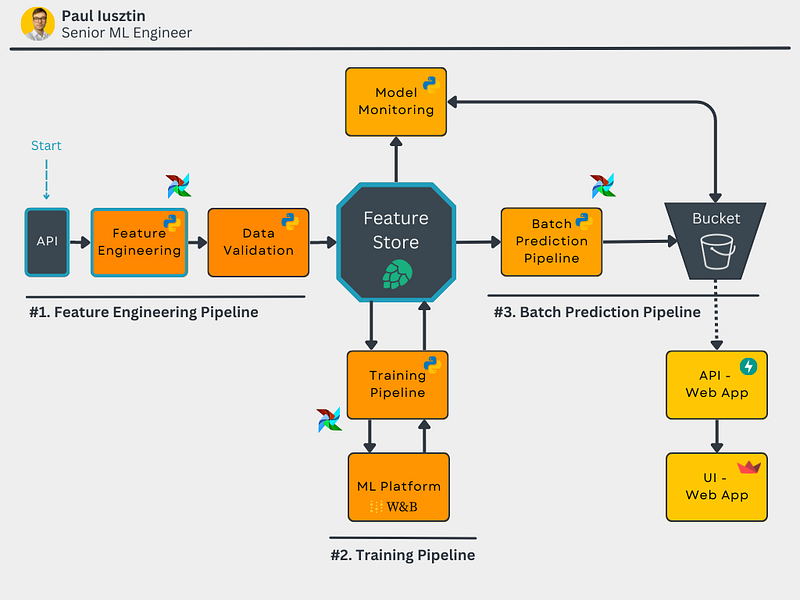
By the end of the course, you will know how to implement the diagram below. Don't worry if something doesn't make sense to you. I will explain everything in detail.

Why batch serving?

There are 4 main types of deploying a model:

• batch serving
• request-response
• streaming
• embedded

Batch serving is the perfect starting point for getting hands-on experience with building a real-world ML system because most AI applications start using batch architecture and move towards request-response or streaming.

Lessons:

1. Batch Serving. Feature Stores. Feature Engineering Pipelines.
2. Training Pipelines. ML Platforms. Hyperparameter Tuning.
3. Batch Prediction Pipeline. Package Python Modules with Poetry.
4. Private PyPi Server. Orchestrate Everything with Airflow.
5. Data Validation for Quality and Integrity using GE. Model Performance Continuous Monitoring.
6. Consume and Visualize your Model’s Predictions using FastAPI and Streamlit. Dockerize Everything.
7. Deploy All the ML Components to GCP. Build a CI/CD Pipeline Using Github Actions.
8. [Bonus] Behind the Scenes of an ‘Imperfect’ ML Project — Lessons and Insights

Data Source:

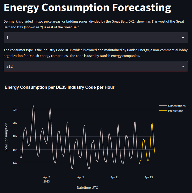
We used an open API that provides hourly energy consumption values for all the energy consumer types within Denmark.

They provide an intuitive interface where you can easily query and visualize the data. You can access the data here [1].

The data has 4 main attributes:

• Hour UTC: the UTC datetime when the data point was observed.
• Price Area: Denmark is divided into two price areas: DK1 and DK2 — divided by the Great Belt. DK1 is west of the Great Belt, and DK2 is east of the Great Belt.
• Consumer Type: The consumer type is the Industry Code DE35, owned and maintained by Danish Energy.
• Total Consumption: Total electricity consumption in kWh

Note: The observations have a lag of 15 days! But for our demo use case, that is not a problem, as we can simulate the same steps as it would be in real-time.

The data points have an hourly resolution. For example: "2023–04–15 21:00Z", "2023–04–15 20:00Z", "2023–04–15 19:00Z", etc.

We will model the data as multiple time series. Each unique price area and consumer type tuple represents its unique time series.

Thus, we will build a model that independently forecasts the energy consumption for the next 24 hours for every time series.

Check out the video below to better understand what the data looks like 👇

Lesson 1: Batch Serving. Feature Stores. Feature Engineering Pipelines.

The Goal of Lesson 1

In lesson 1, we will focus on the components highlighted in blue: "API," "Feature Engineering," and the "Feature Store," as we can see in the diagram below.

Concretely, we will build an ETL pipeline that extracts data from the energy consumption API, pass them through the feature engineering pipeline, which cleans and transforms the features, and loads the features in the feature store for further usage across the system.

As you can see, the feature store stands at the heart of the system.

Theoretical Concepts & Tools

Batch Serving: in the batch serving paradigm, you can prepare your data, train your model, and make predictions in an offline fashion. Afterward, you store the predictions in a database from where a client/application will use the predictions down the line. The word batch comes from the idea that you can process multiple samples simultaneously, which in this paradigm is usually valid. We computed all the predictions in our use case and stored them in a blob storage/bucket.

If we would oversimplify our architecture to reflect only the main steps of a batch architecture, this is how it would look like 👇

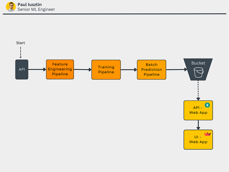
The biggest downside of the batch-serving paradigm is that your predictions will almost always lag. For example, in our case, we predict the energy consumption for the next 24 hours, and because of this lag, our predictions might be 1 hour late.

Check out this article to learn more about a standardized architecture suggested by Google Cloud that can be leveraged in almost any ML system.

Feature Store: the feature store stays at the heart of any ML system. Using a feature store, you can easily store and share features across the system. You can intuitively see a feature store as a fancy database that adds the following features:

• data versioning and lineage
• data validation
• the ability to create datasets
• the ability to hold train/validation/test splits
• two types of storage: offline (cheap, but high latency) and online (more expensive, but low latency).
• time-travel: easily access data given a time window
• hold feature transformation in addition to the feature themselves
• data monitoring, etc...…

If you want to read about feature stores, check out this article [3].

We chose Hopsworks as our feature store because it is serverless and offers a generous free plan that is more than enough to create this course.

Also, Hopsworks is very well designed and provides all the features mentioned above. If you are looking for a serverless feature store, I recommend them.

If you want also to run the code while reading this lesson, you have to go to Hopswork, create an account, and a project. All the other steps will be explained in the rest of the class.

I ensured that all the steps from this course would remain in their free plan. Thus it won't cost you any $$$.

Feature Engineering Pipeline: the piece of code that reads data from one or more data sources, cleans, transforms, validates the data and loads it to a feature store (basically an ETL pipeline).

Pandas vs. Spark: we chose to use Pandas in this course as our data processing library because the data is small. Thus, it easily fits in the computer's memory and using a distributed computing framework such as Spark would have made everything too complicated. But in many real-world case scenarios, when the data is too big to fit on a single computer (aka big data), you will use Spark (or another distributed computing tool) to do the exact same steps as in this lesson. Check out this article to see how Spark can predict churn with big data.

Lesson 1: Code

You can access the GitHub repository here.

Note: All the installation instructions are in the READMEs of the repository. Here we will jump straight to the code.

All the code within Lesson 1 is located under the feature-pipeline folder.

The files under the feature-pipeline folder are structured as follows:

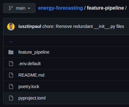
All the code is located under the feature_pipeline directory (note the "_" instead of "-").

Prepare Credentials

In this lesson, you will use a single service, which you will use as your feature store: Hopsworks (for our use case, it will be free of charge).

Create an account on Hopsworks and a new project (or use the default project). Be careful to name your project differently than “energy_consumption,” as Hopsworks requires unique names across its serverless deployment.

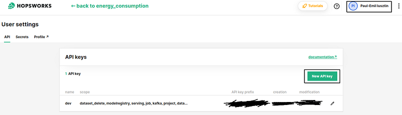
Now, you need an API_KEY from Hopsworks to log in and access the cloud resources using their Python module for this step.

Directly storing credentials in your git repository is a huge security risk. That is why you will inject sensitive information using a .env file. The .env.default is an example of all the variables you must configure.

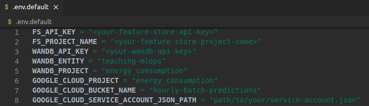
From your feature-pipeline directory, run in your terminal:

cp .env.default .env

…and fill your newly generated Hopsworks API KEY under the FS_API_KEY variable and your Hopsworks project name under the FS_PROJECT_NAME variable (in our case, it was “energy_consumption”).

See the image below to see how to get your own Hopsworks API KEY 👇

Afterward, in the feature_pipeline/settings.py file, we will load all the variables from the .env file using the good old dotenv Python package.

If you want to load the .env file from a different place than the current directory, you can export the ML_PIPELINE_ROOT_DIR environment variable when running the script. This is a "HOME" environment variable that points to the rest of the configuration files.

We will also use the ML_PIPELINE_ROOT_DIR env var to point to a single directory from where to load the .env file and read/write data across all the processes.

Here is an example of how to use the ML_PIPELINE_ROOT_DIR variable:

export ML_PIPELINE_ROOT_DIR=/my/awesome/path python -m feature_pipeline.pipeline

Using the following code, we will have access to all the credentials/sensitive information across our code using the SETTINGS dictionary.

ETL Code

In the feature_pipeline/pipeline.py file, we have the main entry point of the pipeline under the run() method.

As you can see below, the run method follows on a high level the exact steps of an ETL pipeline:

1. extract.from_api() — Extract the data from the energy consumption API.
2. transform() — Transform the extracted data.
3. validation.build_expectation_suite() — Build the data validation and integrity suite. Ignore this step, as we will insist on it in Lesson 6.
4. load.to_feature_store() — Load the data in the feature store.

Please note how I used the logger to reflect the system's current state. When your program is deployed and running 24/7, having verbose logging is crucial to debugging the system. Also, always use the Python logger instead of the print method, as you can choose different logging levels and output streams.

On a higher level, it seems easy to understand. Let's dive into each component separately.

#1. Extract

In the extracting step, we request data for a given window length. The window will have a length equal to days_export. The first data point of the window is export_end_reference_datetime - days_delay - days_export, and the last data point of the window is equal to export_end_reference_datetime - days_delay.

We used the parameter days_delay to move the window based on the delay of the data. In our use case, the API has a delay of 15 days.

As explained above, the function makes an HTTP GET request to the API requesting data. Afterward, the response is decoded and loaded into a Pandas DataFrame.

The function returns the DataFrame plus additional metadata containing information about the data's extraction.

#2. Transform

The transform steps take the raw DataFrame and apply the following transformations:

• rename the columns to a Python-standardized format
• cast the columns to their suited type
• encode the strings columns to ints

Note that we haven't included our EDA step (e.g., looking for null values), as our primary focus is on designing the system, not on the standard data science process.

#3. Data Validation

This is where we ensure that the data is as expected. In our case, based on our EDA and transformations, we are looking that:

• the data doesn't have any nulls
• the types of columns are as expected
• the range of values is as expected

More on this subject in Lesson 6.

#4. Load

This is where we load our processed DataFrame into the feature store.

Hopsworks has a set of great tutorials which you can check here. But let me explain what is going on:

• We login into our Hopsworks project using our API_KEY.
• We get a reference to the feature store.
• We get or create a feature group which is basically a database table with all the goodies of a feature store on top of it (read more here [5]).
• We insert our new processed data samples.
• We add a set of feature descriptions for every feature of our data.
• We command Hopsworks to compute statistics for every feature.

Check out the video below to see what I explained above looks into Hopsworks 👇

Awesome! Now we have a Python ETL script that extracts the data from the energy consumption API for a given time window and loads it into the feature store.

Create a Feature View & Training Dataset

One final step is to create a feature view and training dataset that will later be ingested into the training pipeline.

Note: The feature pipeline is the only process that does WRITES to the feature store. Other components will only query the feature store for various datasets. By doing so, we can safely use the feature store as our only source of truth and share the feature across the system.

In the feature_pipeline/feature_view.py file, we have the create() method that runs the following logic:

1. We load the metadata from the feature pipeline. Remember that the FE metadata contains the start and end of the extraction window, the version of the feature group, etc.
2. We login into the Hopswork project & create a reference to the feature store.
3. We delete all the old feature views (usually, you don't have to do this step. Quite the opposite, you want to keep your old datasets. But Hopwork's free version limits you to 100 feature views. Thus, we wanted to keep our free version).
4. We get the feature group based on the given version.
5. We create a feature view with all the data from the loaded feature group.
6. We create a training dataset using only the given time window.
7. We create a snapshot of the metadata and save it to disk.

Note: A feature view is a smart way of combining multiple feature groups into a single "dataset." It is similar to a VIEW in a SQL database. You can read more about feature views here [4].

That was it. You built a feature pipeline that extracts, transforms, and loads the data to a feature store. Based on the data from the feature store, you created a feature view and training dataset that will later be used within the system as the single source of truth.

Note: You need good software engineering principles and patterns knowledge to build robust feature engineering pipelines. You can read some hands-on examples here.

Important Design Decision

As you saw, we haven't actually computed any features in this lesson. We just cleaned, validated and ensured that the data was ready to be used later in the system.

But this is called "the feature pipeline," why we haven't computed any features?

Let me explain.

a feature = raw data + a transformation function

What if, instead of computing and storing the features, we store the raw data and the transformation functions within the feature store?

Doing so we have the following benefits:

• Faster experimentation, as the data scientist doesn't require to ask the data engineer to compute a new feature. He needs to add a new transformation to the feature store.
• You save a lot of storage. For example, instead of saving 5 features computed from the same raw data column, you save only the raw data column + the 5 transformations, which will use only 1/5 of the space.

Downsides of using this approach:

• Your features will be computed on the cloud or the inference pipeline at runtime. Thus, you will add extra latency at runtime.

But, when using the batch-serving paradigm, latency is not a significant constraint. Thus, we did just that!

Check out Lesson 2 to see how we modeled our time series to forecast the energy consumption for the next 24 hours. In Lesson 2, we will show you how we stored the transformations directly in the feature store.

Conclusion

Congratulations! You finished the first lesson from the Full Stack 7-Steps MLOps Framework course.

You learned about how to design a batch-serving architecture and about developing your own ETL pipeline that:

• extracts data from an HTTP API
• cleans it
• transforms it
• loads it into a feature store
• creates a new training dataset version

Now that you understand the power of using a feature store and its importance to any ML system, you can deploy your model in weeks instead of months.

Check out Lesson 2 to learn about training pipelines, ML platforms, and hyperparameter tuning.

Also, you can access the GitHub repository here.

💡 My goal is to help machine learning engineers level up in designing and productionizing ML systems. Follow me on LinkedIn or subscribe to my weekly newsletter for more insights!

🔥 If you enjoy reading articles like this and wish to support my writing, consider becoming a Medium member. By using my referral link, you can support me without any extra cost while enjoying limitless access to Medium’s rich collection of stories.

References

[1] Energy Consumption per DE35 Industry Code from Denmark API, Denmark Energy Data Service

[2] Hopsworks Tutorials, Hopsworks Documentation

[3] Jim Dowling, Feature Store vs Data Warehouse (2020), KDnuggets

[4] Hopsworks Feature Views, Hopsworks Documentation

[5] Hopsworks Feature Groups, Hopsworks Documentation