A Deep Learning Approach in Predicting the Next Word(s)

Teaching a computer to predict the next set of words in a sentence

In this tutorial, we will walk through the process of building a deep learning model used to predict the next word(s) following a seed phrase. For example, we’ll ask the computer to predict the next 10 words after we have typed “The candidates are”.

Although cutting-edge models used in your smartphones to assist with sending text messages are vastly more complex, this article should give you a general idea of the methodology involved in this prediction (classification) task.

This article will review:

1. Text Processing: tokenization, n_gram sequencing, engineering features and labels, and word embeddings
2. Building a Bidirectional LSTM model
3. Using our model to predict words based on a seed phrase

Let’s Code!

All development for this tutorial has been done using Google Colab for its data processing capabilities. You can certainly run this code on your local machine but unless you have a dedicated GPU the training times might be rather lengthy.

For this tutorial, we’ll use snippets of users’ comments on New York Times articles LINK. As this is merely a tutorial and natural language data is extremely computationally expensive the limited scope of this dataset suits our needs very well.

Let’s load the required libraries and since the training data resides on Google Drive we’ll mount gdrive to Colab. Finally, we’ll change our directory to where our training data resides. Be aware that linking your Google Drive with Colab will automatically create the “Colab Notebooks” directory in your Google Drive. Due to the space between “Colab” and “Notebooks” your path directory might be slightly different. For example, notice the backward-slash used to designate a space “/content/drive/MyDrive/Colab\Notebooks”

import csv
import nltk
import string
import pandas as pd
import numpy as np
from google.colab import drive
from keras import backend as K
import tensorflow as tf
from tensorflow.keras.preprocessing.sequence import pad_sequences
from tensorflow.keras.layers import Embedding, LSTM, Dense, Bidirectional
from tensorflow.keras.preprocessing.text import Tokenizer
from tensorflow.keras.models import Sequential
from tensorflow.keras.optimizers import Adam

drive.mount('/content/drive/')

%cd '/content/drive/MyDrive/Colab Notebooks'

Determining what data will be used to train our deep learning model is very important. You obviously wouldn’t want to train your model using Shakespeare’s writing when trying to build a modern-day text prediction model. Your model would learn the contextual nuances amount the words as written by Shakespeare which would not effectively translate to today’s modern English. Using a dataset which is most likely to reflect the type of sentences you wish to predict will yield the best results. That said, utilizing very large datasets of generalized text, think Wikipedia, can also produce accurate results.

We’ll use Pandas to read in the CSV file and print out the first 5 rows. We’ll be using the highlighted “snippet” column which contains an excerpt of the comments left by the user. Our data has a strong political and global news connotation but for this tutorial, this will suffice.

path = '/content/drive/MyDrive/Colab Notebooks/ArticlesMarch2018.csv'

df = pd.read_csv(path)

df.head()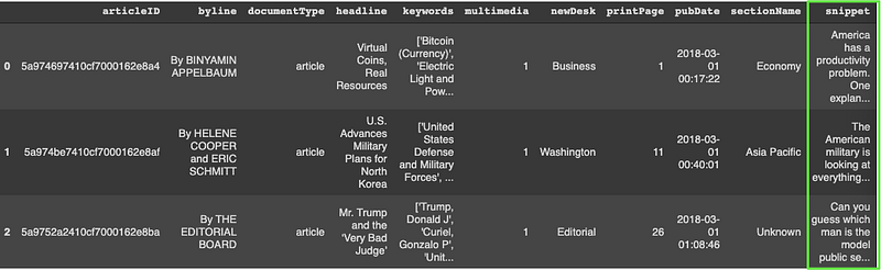

Text Processing

We need to apply a few processing steps to our data before building our model. First, let’s combine all the snippets into a series of strings.

snippet = '\n'.join(df['snippet'])

print(type(snippet))

print(snippet)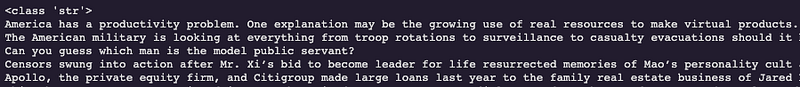

Next, we’ll transform any capitalized word into lowercase to reduce the size of our vocabulary. Otherwise, we would have duplicate words, the only difference being the capital letter (ie. America/america). Notice the lower() function has transformed our string into a list of strings.

Our corpus contains 1,385 unique snippets.

corpus = snippet.lower().split('\n')

print(len(corpus))

print(type(corpus))

print(corpus[:2])

Tokenizer

As computers cannot process raw text data, we need to tokenize our corpus to transform the text into numerical values. Keras’s Tokenizer class transforms text based on word frequency where the most common word will have a tokenized value of 1, the next most common word the value 2, and so on. The result is a dictionary containing key/value pairs of the unique word and its assigned token determined based on word frequency.

We have 6,862 unique words in our vocabulary plus (1) for out of vocabulary words. Notice that Keras’s Tokenizer class automatically removes all punctuation from our corpus. Often, when dealing with NLP prediction tasks we remove what are called “stopwords” or terms which really don’t add much meaning to a sentence (ie. the, he, in, for, etc.). However, as we are trying to predict sentences which resemble human speech we’ll keep the stopwords.

tokenizer = Tokenizer()
tokenizer.fit_on_texts(corpus)
word_index = tokenizer.word_index
total_unique_words = len(tokenizer.word_index) + 1 

print(total_unique_words)
print(word_index)

Although the code below is not necessary for our analysis, it is good practice to compare the actual text along with its tokenized version for accuracy.

We can see our entire tokenized corpus by applying the code below. For example, the first snippet starts with “america has a productivity problem” which has been tokenized to [193, 14, 2, 2796, 699]. Examining the word_index dictionary above, we see that the letter “a” has been tokenized with the number 2 which corresponds with the tokenized first snippet.

for line in corpus:
   seqs = tokenizer.texts_to_sequences([line])[0]

print(seqs)

N_Grams

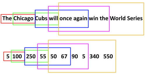
Here comes a tricky portion of this tutorial. In typical supervised regression or classification problems our dataset would contain the x_values (ie. input features) and y_values (ie. labels) which allows the model to learn the unique patterns among our features in relation to our labels. Our dataset seems to be missing the y_values (ie. labels). Fear not, n_grams help assist us in splitting our data in order to derive our labels. An n_gram is a sequence of words (n) sizes long. For example, “Chicago Cubs are” is an n_gram of length 3 (ie. 3_gram).

Many-to-One N_Gram Sequences

We are going to take this concept one step further and iterate over each tokenized snippet to create n_grams the size of n_gram+1. Sometimes this is called a “many-to-one” sequence map. For example, our first five tokenized words in the first snippet (ie. america has a productivity problem) are [193, 14, 2, 2796, 699]. By creating n_gram+1 sequences of n_grams we produce the list below.

We use this approach for all snippets which eventually yields almost 27,000 n_grams. Let’s examine the code in a bit more detail. First, we create an empty list which will hold our n_gram sequences described above. Next, we iterate over our corpus of untokenized snippets and apply the “texts_to_sequences” method to each untokenized snippet. As we saw above, the “texts_to_sequences” method simply converts each snippet to its tokenized version. Next, we iterate over each token beginning with the second (index=1) thru all remaining tokens. At each iteration, we append the sequence of n_grams to input_sequences and expand the n_gram+1.

input_sequences = []

for line in corpus:
  token_list = tokenizer.texts_to_sequences([line])[0]
    for i in range(1, len(token_list)): 
      n_gram_seqs = token_list[:i+1]
      input_sequences.append(n_gram_seqs)

print(len(input_sequences))
print(input_sequences)

Padding of N_Grams

Notice that the n_grams are of different lengths and our model requires each input sequence of n_grams to be of the same length. Therefore, we need to “pad” each n_gram sequence with zeros to the length of the longest n_gram. Max_seq_length will identify the length of the longest n_gram sequence (ie. 41). Then the “pad_sequences” method will add zeros prior to our tokens (ie. padding=’pre) to the length of max_seq_lenth (ie. 41).

max_seq_length = max([len(x) for x in input_sequences])
input_seqs = np.array(pad_sequences(input_sequences, maxlen=max_seq_length, padding='pre'))

print(max_seq_length)
print(input_seqs[:5])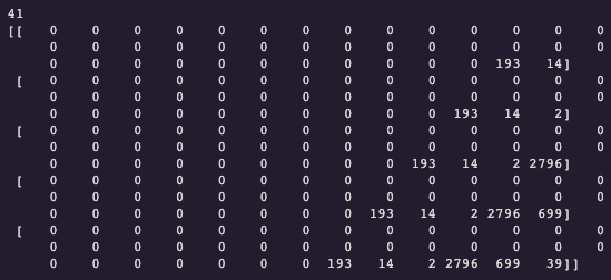

Creating Features and Labels

Now that we have padded created and padded our n_gram sequences we can extract our features and labels. Recall that each n_gram sequence is 41 values in length. The first 40 values will be our features and the 41st value will be our label. In theory, this is a multi-class classification problem as the model will learn the relationships among our words and then provide probabilities as to which word should be next in our sequence. The model can only provide probabilities for words it has seen (ie. total number of unique words: 6,863). Since this is a multi-classification problem, we’ll apply one-hot encoding for our labels as well. Below we have printed the first three features and labels (without one-hot encoding) to demonstrate our methodology.

x_values, labels = input_seqs[:, :-1], input_seqs[:, -1]

y_values = tf.keras.utils.to_categorical(labels, num_classes=total_unique_words)\

print(x_values[:3])
print(labels[:3])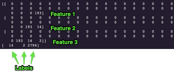

Our one-hot encoded labels (ie. y_values) have a shape of 26,937 (ie. the number of sequenced n_grams) by 6,863 (ie. the number of unique words in the corpus). Each word in our corpus, except the first word, is both a feature and a label as the model will learn what words are more and less likely to follow other sequences of words.

Word Embeddings

The name of the game in these types of NLP problems is “context”. How can we optimize our strategy (ie. data processing and model complexity) to enable our model to be better able to learn the relationships among words. In its current form, our data is providing forward context for our model to learn. In other words, we know what words are more or less likely are to follow other words due to our n_gram sequences. However, the tokens used to represent each word are nothing but frequency counts which provide the model limited information regarding the contextual information among the words. For example, words such as “good” and “great” are very similar in meaning yet their respected token values are (299, 673).

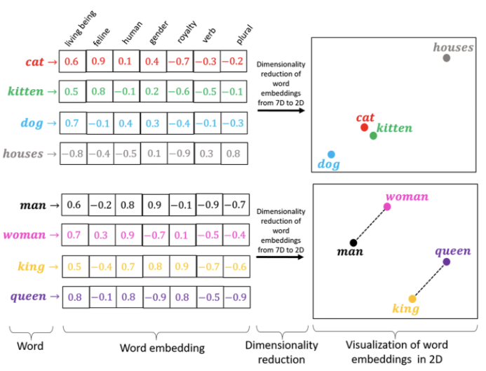
print(tokenizer.word_index['good'])

print(tokenizer.word_index['great'])

Word embeddings enable us to represent words in a n_dimensional space where words such as “good” and “great” have similar representations in this n_dimensional space which the computer can understand. In the image below we can see word embeddings (7-dimensional) for words such as dog, puppy, cat, houses, man, woman, king, and queen. The dimensions are unknown to us (not interpretable) as the model learns these dimensions as it iterates over the data. That said, to aid the reader in an understanding of word embeddings models, let’s assume the dimensions are “living being, feline, human, gender, royalty, verb, plural”. We can see that “houses” have a -0.8 embedding on D1 (ie. living being) whereas all other words score relatively high on the “living being” dimension. By learning these embeddings the computer is better able to understand the contextual relationships among words and therefore should be better able to predict the next word(s) following a seed phrase.

Keras has an “Embedding” layer that can build its own word embeddings based on our corpus but we will utilize a pre-trained word embeddings model from Stanford University named “GloVe” (Global Vectors for Word Representation). The GloVe embeddings come in several flavors but we’ll use the 100-dimensional version. You will need to download the pre-trained model from this link. This model was trained on a billion words with a vocabulary (ie. unique words) of 400 thousand words.

First, let’s process the embeddings text file and produce a dictionary which contains the word/character as the key and a 100-dimensional array as the value.

path = '/content/drive/MyDrive/Colab Notebooks/glove.6B.100d.txt'

embeddings_index = {}

with open(path) as f:
  for line in f:
    values = line.split()
    word = values[0]
    coeffs = np.array(values[1:], dtype='float32')
    embeddings_index[word] = coeffs

dict(list(embeddings_index.items())[0:2])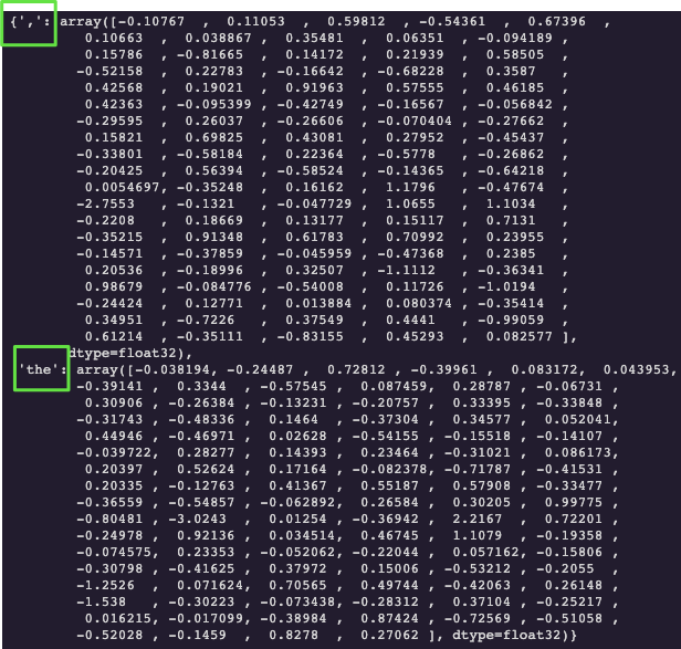

Now let’s create a matrix which contains the GloVe word embeddings (ie. 100-dimensional arrays) only for the words in our vocabulary. First, we create a matrix of zeros with the shape of 6,863 (ie. total number of unique words in our corpus) by 100 (ie. glove contains 100 dimensions). Then we are going to iterate over the “word_index” dictionary which contains the unique words in your corpus as the keys and their corresponding tokens as the values. At each iteration through the word_index dictionary, we’ll fetch the corresponding GloVe embeddings (ie. 100-dimensional array) stored in “embeddings_index” and update the embeddings_matrix (ie. replace the zeros with the 100-dimensional array).

embeddings_matrix = np.zeros((total_unique_words, 100))

for word, i in word_index.items():
   embedding_vector = embeddings_index.get(word)
   if embedding_vector is not None:
     embeddings_matrix[i] = embedding_vector;

Building our Model

We’ll build a relatively shallow model consisting of an embedding layer, three LSTM layers, three dropout layers, and a fully connected Dense layer. The first layer being the Embedding layer will enable us to utilize the pre-trained GloVe word embeddings coefficients/weights. The embedding layer requires an input_dim of the total number of unique words (ie. size of vocabulary) in your corpus and an output_dim which specifies the number of word embedding dimensions we want. As we are using GloVe 100-dimensions our out_dim parameter will be 100. We’ll pass the embeddings_matrix into the weights argument in order to use the GloVe weights and set the trainable argument to “False”, otherwise, we’ll retrain the GloVe weights. Finally, we’ll set the input_length parameter to “max_seq_length -1”.

Recurrent Neural Networks

Recall that helping your model to understand the context or the relationships among the words will ultimately yield a better-performing model. We have used n_gram sequences and word embeddings to assist our model in learning these relationships. We can now utilize a specific model architecture particularly suited to examine the relationships among sequences of words. In traditional neural networks, the input and predictions/outputs are completely independent of each other. On the other hand, we are trying to predict the next word in a sentence which means the network needs to “remember” the contextual information from previous words.

A Recurrent Neural Network (RNN) model architecture incorporates previous data to make future predictions. In other words, RNNs have a built-in memory function which stores information from previous words and uses that information when predicting the next word. That said, simple RNNs have trouble “remembering” information learned earlier in the sequence. In other words, given a sentence of words, an RNN can incorporate the information among a few adjacent words but as the RNN continues to iterate over the sentence the relationships between the first and the latter words in the sentence begin to lose their meaning. This is particularly important when you have a very deep model contain dozens or hundreds of hidden layers.

A Long Short-Term Memory (LSTM) model gets around this issue by learning the relationships among words and allowing the important relationships to propagate through the network. This way the information learned during the first few words in a sequence can influence the prediction further in the sequence/sentence, paragraph, chapter, etc. What’s more, we will utilize a Bidirectional LSTM which will learn the relationships among words reading the sentence from left-to-right and right-to-left.

The input to our LSTM layers is always 3-dimensional (ie. batch_size, max_seq_length, num_features). The batch_size will be set to None which simply specifies the layer will take any size of a batch. Max_seq_length is 40 as all snippets have been tokenized and padded to 41 minus 1 as our label. Finally, we have 100 features because GloVe has 100 dimensions.

We’ll add three dropout layers (drop 30%) to help with overfitting the model to training data.

Deep learning is an exercise in futility as you can adjust parameters for the rest of time. Choosing the correct optimizer is just another parameter we can tweak. We ultimately settled on Adam as it outperformed SGD and RMSProp both in terms of outright model accuracy and efficiency as the loss decreased almost twice as fast compared to SGD and RMSProp.

Since the output of this model can be 1 out of 6,863 (ie. total_unique_words) words, this is a multi-class classification problem which is why we are using categorical_crossentropy as our loss function.

K.clear_session()

model = tf.keras.Sequential([

tf.keras.layers.Embedding(input_dim = total_unique_words, output_dim=100, weights=[embeddings_matrix], input_length=max_seq_length-1, trainable=False),

tf.keras.layers.Bidirectional(tf.keras.layers.LSTM(256, return_sequences=True)),

tf.keras.layers.Dropout(0.2), 

tf.keras.layers.Bidirectional(tf.keras.layers.LSTM(256)),

tf.keras.layers.Dropout(0.2),

tf.keras.layers.Dense(128, activation='relu'),

tf.keras.layers.Dense(total_unique_words , activation='softmax')])

model.compile(optimizer=Adam(learning_rate=0.001), loss='categorical_crossentropy', metrics=['accuracy'])

tf.keras.utils.plot_model(model, show_shapes=True)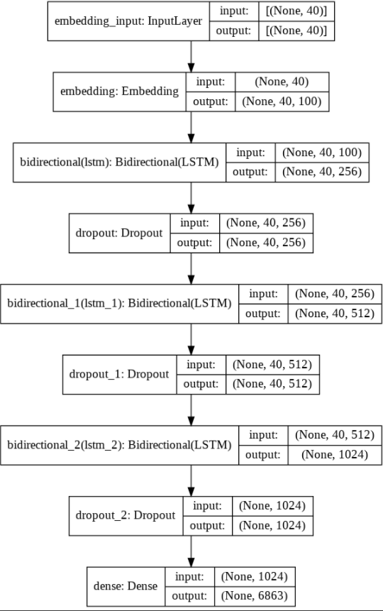

Finally, we’ll fit/train our model using the x_values and y_values. Selecting the batch_size is yet another parameter we can tweak to. Since we have 26,937 n_grams to train our model it would be very inefficient to load all 26,937 n_grams at once. Let’s train our model for 120 epochs where 1 epoch requires all 26, 937 n_grams to run through the model once. Therefore, 26,937 (ie. 27,000) divided by 120 means each batch_size should be 225 n_grams. However, to best utilize our memory, we’ll use a batch_size of 256. We’ll also apply an 80/20 split for training and validation data.

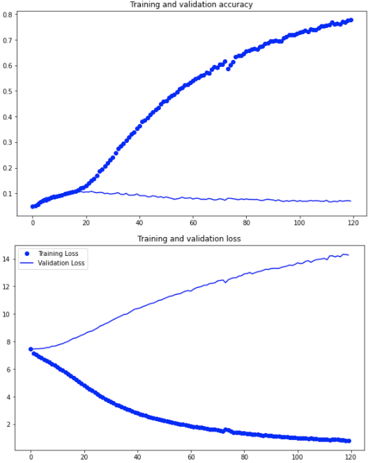
history = model.fit(x_values, y_values, epochs=120, validation_split=0.2, verbose=1, batch_size=256)

Model Evaluation

Our model is definitely overfitting our training data as training accuracy continues to increase whereas validation accuracy has plateaued. Well-performing NLP models are very data-hungry. It is not unusual to see datasets with tens of millions of words whereas our corpus consisted of merely 6,863 words. We can add additional LSTM layers, more regularization techniques along with more data to improve the model but this tutorial is meant to you give, the reader, a general idea of how to structure and build word prediction models. With that said, let’s see how well our model predicts actual new snippets.

Seed Text Prediction

Let’s examine how well our model can generalize to news snippets which it hasn’t seen before. We’ll seed the model with the first few words of each actual news snippet from the previous month and compare the model’s prediction.

def prediction(seed_text, next_words): 
  for _ in range(next_words):
  token_list = tokenizer.texts_to_sequences([seed_text])[0]
  token_list = pad_sequences([token_list], maxlen=max_seq_length-1, padding='pre')

  predicted = np.argmax(model.predict(token_list, verbose=1), axis=-1)

  ouput_word = ""

  for word, index in tokenizer.word_index.items():
    if index == predicted:
      output_word = word
      break
  seed_text += ' '+output_word
  print(seed_text)

seed_phrase = "I understand that they could meet"
next_words = len("with us, patronize us and do nothing in the end".split())

prediction(seed_text, next_words)

The model generated text is certainly oriented around global news and politics. We see words such as “generation”, “government”, “borrow”, “regulation”, “policies” which fits the type of data the model learned. Unfortunately, it is not difficult to identify model generated text from human snippets. Furthermore, when we used a seed phrase with a very different context “I truly enjoy riding my motorcycle” the model had a particularly difficult time classifying a sentence that resembles an accurate English sentence.

Actual News Snippet 1

“I understand that they could meet with us, patronize us and do nothing in the end”

Seed Phrase 1

“I understand that they could meet”

Model Generated 1

“I understand that they could meet the defining challenge of your generation and why you borrow”

Actual News Snippet 2

“The agency plans to publish a new regulation Tuesday that would restrict the kinds of scientific studies the agency can use when it develops policies.”

Seed Phrase 2

“The agency plans to publish a new regulation Tuesday that would restrict the”

Model Generated 2

“The agency plans to publish a new regulation Tuesday that would restrict the government through september what happens happens happens they must be the third”

Actual News Snippet 3

“Gun owners who favor increased restrictions can be an overlooked group. Some have grown more vocal, marching and testifying in favor of limits.

Seed Phrase 3

“Gun owners who favor increased restrictions”

Model Generated 3

Gun owners who favor increased restrictions for experts are recently in a plan to introduce sweeping tariffs on steel and aluminum tariffs while

Self Generated Seed Phrase

“I truly enjoy riding my motorcycle”

Model Generated Phrase

“I truly enjoy riding my motorcycle list yet everyone asks i hate this question”

Conclusion

This is certainly an exciting time in the world of natural language processing. Models such as OpenAI’s “GPT-3” are continuing to push the advancement of our NLP capabilities. This tutorial served as a rather simple introduction to text classification and I hope it inspired your interest in this exciting area.

Some insights into OpenAI’s GPT-3 capabilities LINK.