Hands-on Tutorials

A Comprehensive Beginner’s Guide to the Diverse Field of Anomaly Detection

Isolation Forest, Local Outlier Factor, One-Class SVM, Autoencoders, Robust Covariance Estimator and Time Series Analysis

Anomaly or outlier detection deals with the detection of patterns in data that do not correspond to the expected behavior. The methods are used in almost all industries. Well known areas of application are the detection of credit card and insurance fraud, cybersecurity, monitoring of security-relevant systems and the assessment of military activities. [Cha09a]

Since I will be using an example from production in the course of the article, I do not want to leave this important area of application unmentioned here either. Smart Factories are becoming increasingly agile, more flexible, more variable and thus more complex [Eur10]. Due to this constantly growing complexity, operators have trouble to monitor processes and identify deviations. Problems and failures are often detected too late, maintenance intervals are not chosen correctly [Win15]. Intelligent systems for early detection of anomalies can offer significant relief by detecting deviations at an early stage and avoid production downtimes.

The article is intended to give you an overview of the field of anomaly detection and used techniques by answering the following questions:

• What are the types of anomalies? How can they be characterized?
• Which procedures and methodologies are used to identify anomalies in datasets? How can they be distinguished from each other?
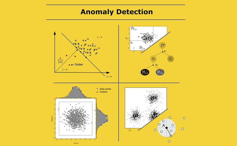
• What specific algorithms are used, and how do they work? - Robust Covariance Estimator - Isolation Forest - Local Outlier Factor - One-Class Support Vector Machine - Autoencoders - Time Series Analysis

Please don’t get confused by the terms “anomaly” and “outlier”, I will use both as synonyms for each other.

Types of Anomalies

Anomalies differ decisively in their occurrence. Basically, anomalies can be divided into three types:

• Point/Global Anomalies
• Collective Anomalies
• Contextual Anomalies

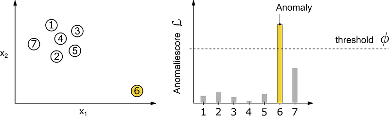
Point Anomaly

Is it able to classify a single instance of data as anomalous with respect to the rest of the data, it is called as a Point or Global Anomaly. This describes the simplest type of outliers and is the focus of most publications.

In the following image, the Point Anomaly shows up as a single outlier in a two-dimensional space. The dataset can be clearly divided into 3 clusters. Since the marked data point cannot be assigned to any of the clusters, it must be assumed that this data point represents an Anomaly.

Contextual Anomaly

If an instance appears to be anomalous only in a specific context, it is called a Contextual Anomaly. The context is determined by the structure of the dataset given. [Cha09a]

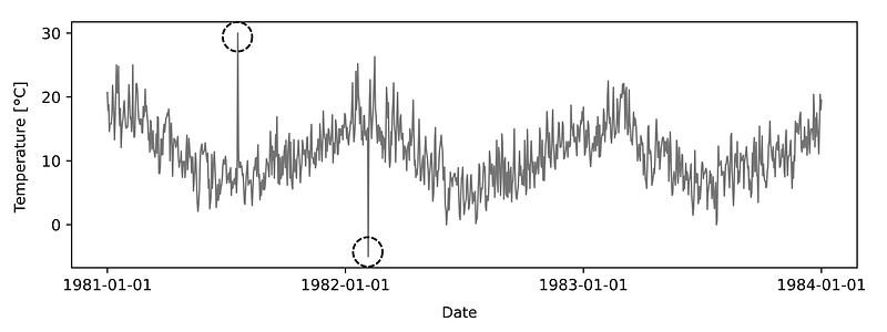
The dataset below shows the temperature trend over the years 1981 to 1984 in Melbourne. The marked data points represent a Contextual Anomaly. Contextual because the temperatures of about 30 and -5 degrees are not unusual per se, but in context to the rest of the course, these instances can be classified as very unlikely. A temperature in the minus range during the summer months, as well as 30 degrees in winter is just very unlikely.

Collective Anomaly

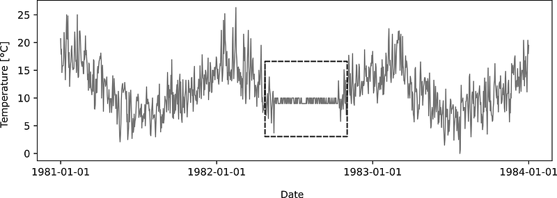
If a collective of related instances can be identified as anomalous to the rest of the dataset, these instances describe a so-called Collective Anomaly. Looking at these instances individually compared to the rest of the dataset, these instances may not be recognized as an anomaly, but their occurrence in the collective justifies a designation as an outlier. [Cha09b]

The following example simulates this with a collective of temperature measurements over several months at approximately the same level.

Which approaches are used to identify anomalies?

The field of Anomaly Detection tries to identify instances of a dataset that are unusual or differ significantly from the majority of the data. [Zim18]. This usually refers to data that deviates from an defined distribution model. The best known distribution function is the normal distribution, which can be used to describe the distribution of measured values for many economic and engineering processes with very good accuracy. [Fah16, p.83][Zim18]

In addition to these probabilistic methods, there are approaches based on decision trees, distance/density methods and reconstruction techniques.

Also supervised methods can play a major role

Especially for labeled training data also model-based methods can be a powerful alternative. Most technical processes are cyclical and are thus represented by recurring signal patterns, patterns which can be modeled with a Regression or Time Series Analysis. This makes it possible to identify even small deviations from the “normal” process.

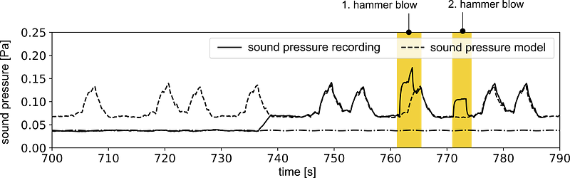
The graph below gives you an example. It shows the airborn sound level recording next to a running milling machine. As in many automated processes, a cyclic signal can be detected (in this case it repeats approximately every 40 seconds). This repetitive signal can be reproduced with high accuracy by time series models. By simply comparing the prediction and recording, this model-based approach can achieve significantly higher accuracy than unsupervised methods. It is definitely helpful here if the training dataset contains no, a small or known number of outliers.

The image shows the formed model of the signal. In this simple case, the deviations are simulated with a hammer blow in the vicinity of the machine. This deviation can be clearly seen by comparing the model and the actual-signal. This approach can be extended with different features like the frequency analysis.

So if you want to detect deviations from recurring signal patterns, modeling the signal is often a powerful approach.

The approaches of the algorithms used differ fundamentally

The following listing tries to classify the different methods. Nevertheless this should not to be seen as a rigid grouping, since different techniques are using approaches from different areas.

• Probabilistic method These approaches are based on certain probabilistic assumptions about the occurrence of events. Data points are evaluated with respect to their probability distribution. Instances with a very low probability are identified as Outliers. (e.g. Robust Covariance Estimator) [Aig15, p.392][Spe14][Ott18]
• Distance and density method Parameter-free methods consider and evaluate data points with respect to their environment. If there are enough similar data points in the area around one data point, the data is evaluated as normal. This similarity of the data is usually represented by the distance between the data points. The k-Nearest-Neighbor-Algorithm works according to this principle. [Ert16, p.207] [Ott18]
• Clustering method These methodes look for grouping of similar objects and structures. The instances are divided into groups in such a way that the data within a group is as similar as possible, but the data of different partitions differ as much as possible from each other. Instances that cannot be assigned to any group are classified as outliers. [Sha13][Hot04]
• Reconstruction method These methods attempt to detect patterns in the data, with the goal of being able to reconstruct the signal without noise. Known algorithms that belong to these methods are Principal Component Analysis (PCA) and Replicator Neural Networks (RNN).

As already mentioned, most approaches aim at modeling the regions in the feature space, which describe the normal behavior of the considered process. Data that lie outside the defined region are called anomalous. However, some factors pose challenges to this relatively simple approach. In practice, it is usually not possible to clearly define the normal range, the boundaries between normal and anomalous behavior are not always clear.

The set of all instances of normal and anomalous behavior, can be described by corresponding probability distributions. Only rarely are these distributions clearly separated from each other and allow a unique classification of normal instances and anomalies. The following image shows the case for most use cases (left) and the target optimal case (right). In the left figure, a 100% correct classification is not achievable.

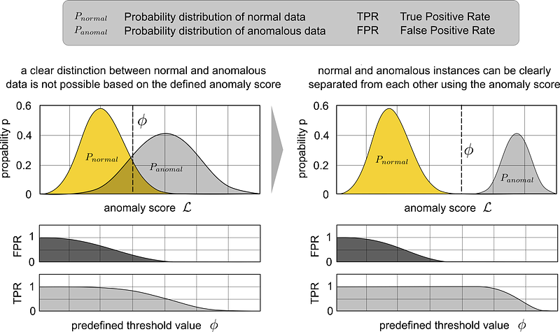
In the case of the left figure, only a maximization of the true-positive and a minimization of the false-positive rate can be aimed at. The right figure shows the goal of an optimal feature extraction. If the features are chosen in such a way that normal and anomalous instances differ strongly from each other, there is no direct intersection of the distribution curves. In this case, the sensitivity can be chosen such that the true-positive rate is 1 and the false-positive rate is 0.

For the already used example of sound pressure recording, acoustics already offers some possibilities of feature transformations e.g. the Fast Fourier Transformation. Converting the signal into the frequency domain can help to distinguish between normal and anomalous events more accurate.

Anomaly detection algorithms evaluate individual data points with an anomaly score, which serves as the basis for subsequent decision-making. Based on a predefined threshold, instances are classified as normal or anomalous with respect to their anomaly score.

The threshold value determines how sensitive the system reacts to anomalous conditions and represents a hyperparameter. While in medicine even small deviations from the normal state can have a great impact and thus must be recognized as an anomaly [Cha09a][Hod04], too high a sensitivity of the systems in the production environment is inappropriate due to a high number of random perturbations. Especially these stochastic influences in the environment of the considered area lead to large noise components in the data, which often resemble anomalies and lead to misclassifications. [Hod04]

For each use case, an evaluation of the consequences of misclassification should be performed. The False Positive Rate (FPR) and True Positive Rate (TPR) are necessarily in a trade-off with each other. The threshold value describes a limit value for the anomaly score. If the anomaly score of a data point exceeds the predefined threshold, it is marked as anomalous. Basically, a decreasing threshold leads to both an increasing TPR and increasing FPR. For most use cases, this is where a trade-off occurs.

Additional knowledge about the process is required to determine the optimal threshold value. In industry, the primary goal is a cost-optimal threshold. For example, an undetected anomaly can lead to equipment failure and repair work. On the other side, a system with high False-Positive Rate leads to a great deal of control effort by operators. To explain this trade-off, the literature often uses a healthcare example. In cancer detection tests, a low threshold is appropriate. Failure to detect early-stage disease reduces the patient’s likelihood of survival, whereas failure to detect the test in a healthy patient merely leads to further testing. Thus, a high TPR is weighted higher than a low FPR.

Novelty vs. Outlier Detection

In the field of anomaly detection, the literature distinguishes between novelty and outlier detection [Sci19b]:

Outlier Detection

If a training dataset contains instances that differ strongly from the rest of the data, these can be attributed to errors in data acquisition, for example. For model building, these data points are disturbing and can negatively influence the model. They should be identified beforehand and removed from the training dataset. [Koi18]

Novelty Detection

Novelty detection assumes that the training dataset contains no or a known number of outliers and is instead interested in whether a new instance describes an anomalous event. [Koi18]

Algorithms used for anomaly detection

A wide variety of algorithms, methodologies and approaches are used for anomaly detection. The following is a compilation of identified methods in this area:

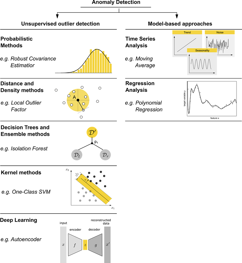
Popular algorithms in the field of anomaly detection are the Robust Covariance Estimator, the Isolation Forest, the Local Outlier Factor Algorithm and the One-Class Support Vector Machine, which will be introduced shortly in the following. In the field of Deep Learning, Autoencoders are primarily used. With the help of time series and regression analyses, models are set up which can reproduce and predict the behavior of a process under consideration.

Robust Covariance Estimator

Many statistical procedures require an estimate about the distribution of the data in terms of a covariance matrix. [Sci19a]

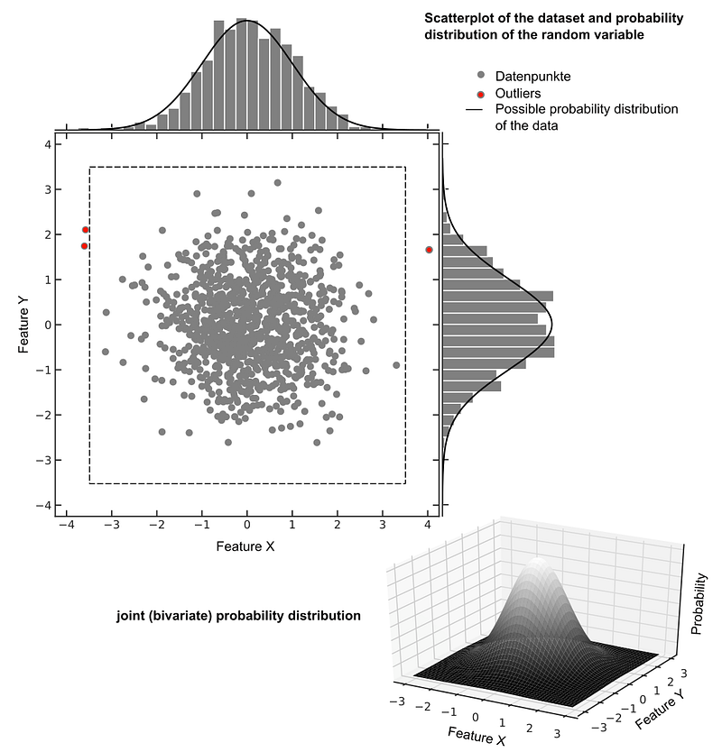
The Joint Probability Distribution describes the probability with which certain combinations of values occur. Given a dataset with two random variables X and Y, the result is a bivariate probability distribution. For several random variables a so-called multivariate distribution. [Haz02][Fer03]

The Robust Covariance Estimator algorithm, often used for Anomaly Detection, detects outliers in datasets by assuming a normal distribution of the data. For new data points, the probability of the measured value can be determined based on the modeled probability distribution.

The most frequently used distribution model is the multivariate normal distribution (Gaussian distribution). The figure below shows a bivariate normal distribution of the two random variables X and Y, with the maximum at x = 0, y = 0. The further away the measured data points lie from this point, the less likely it is that the data point represents the normal behavior of the process under consideration. If the predicted probability of a data point falls below a defined threshold, it is marked as an outlier.

Isolation Forest

The creation of a decision tree is done iteratively by dividing the data at so-called leaf nodes. This division of the data starts at the root of the tree. In regression and classification tasks, the goal with each step is to maximize the information gain IG. This is the case when the splitting of the dataset at a node is done in such a way that the largest reduction of impurity in the child nodes is achieved. Different definitions exist for impurity. Regression for example uses mean squared error, classification uses entropy or the gini coefficient as a measure of impurity. [Ras18, p.107][Has09, p.587][Ras18, p.347]

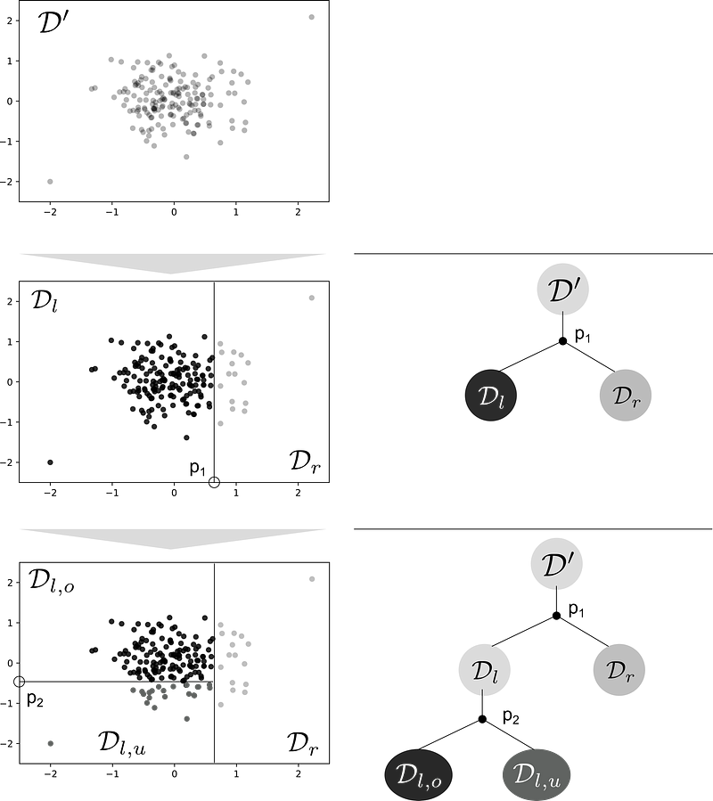
Isolation Trees, on the other hand, splits the dataset randomly. The creation of an Isolation Forest involves the following steps [Har18][Vie19][Liu12]:

1 — For modeling a single Isolation Tree, a subset D′ of size ψ is first selected from the training dataset D in the d-dimensional feature space (D ⊂ R^d)

2 — This partial dataset is used to build an Isolation Tree T ′. For the first partitioning process, the algorithm chooses a random feature q and a partitioning point p, where p is in the range between the maximum and minimum value of the feature in the dataset.

3 — At this division point p the dataset divides into D_l and D_r

4 — Step two and three are repeated until every node has only one instance or all data at the node have the same values

The following figure shows the first two division processes in growing an Isolation Tree for a two-dimensional dataset.

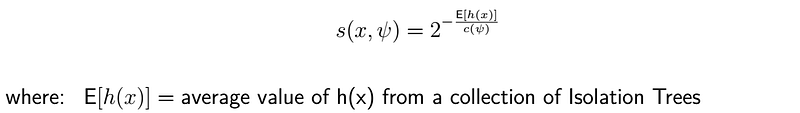
After setting up the Isolation Trees, the method counts the division steps that were required until the individual points were isolated. The algorithm is based on the assumption that significantly fewer steps are required to isolate outliers. The outlier detection is interested in the anomaly score s(x, ψ) of individual data points x, which is described by the path length to isolate a data point.

The following figure shows this procedure for a simple example. While only two division steps are required to isolate data points 1 and 7, instances 5 and 3 are isolated after four division steps. If the creation of the Isolation Tree were to be repeated infinitely often, the number of steps required on average to isolate 6 and 7 would be significantly lower than for the remaining data points.

From Isolation Tree to Isolation Forest

Parts of the entire dataset are used to create each Isolation Tree. With k-different parts of the dataset k-Isolation Trees T_k are created. The result of the Isolation Forest is an average of the path lengths h(x) of the individual Isolation Trees.

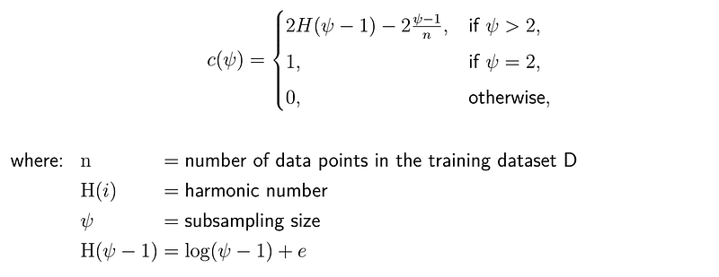
Since the maximum size of the individual isolation trees strongly depends on the size of the dataset D′ used, a normalization is required for a meaningful and comparable result. For this purpose, the normalization factor c(ψ) is introduced, which describes the average path length of unsuccessful searches [Liu12]:

The anomaly score s can then be calculated as:

A more detailed description of how the Random Forest works can be found in the paper “Isolation-based Anomaly Detection”. [Liu12]

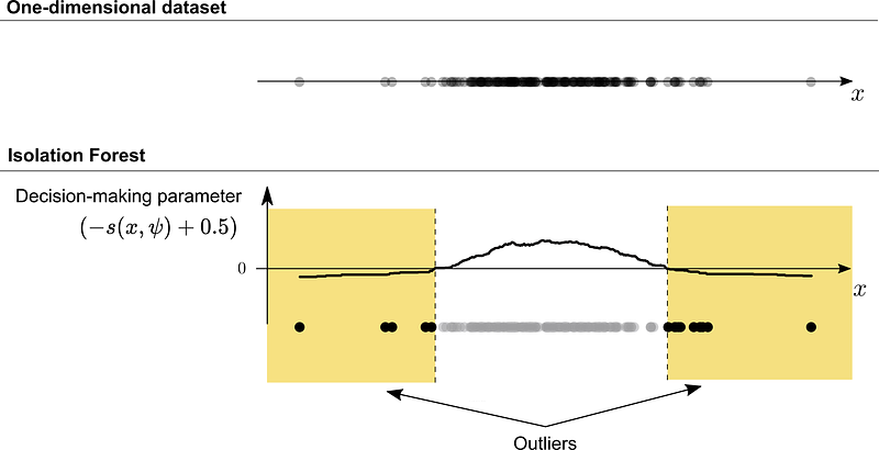
The figure below shows the prediction output of the skicit-learn Isolation Forest module (sklearn.ensemble.IsolationForest ) for a one-dimensional dataset. The graph shows the output of the defined decision function (decision_function = -s — offset_ ), which is calculated using the negated anomaly score s and a defined offset. In this case, the default offset value of -0.5 is used. Thus, the assessment of the data points is as follows: The lower the value, the more abnormal. Negative values are declared as outlier, positive as inlier.

Local Outlier Factor

The Local Outlier Factor (LOF) algorithm finds outliers by measuring the local deviations to a given data point. The algorithm is based on a concept of local point density. The density is described by distance to the k-nearest neighbors. By comparing the density of each instance, regions with similar density can be identified. At the same time, outliers can be detected that show significantly lower density values.

The LOF is one of the methods of density-based clustering, which describe clusters as areas in which objects are located close to each other. For objects in a cluster, the local point density exceeds a given threshold. The set of objects belonging to the same cluster are spatially grouped together.

A commonly used algorithm in this area is DBSCAN (Density-Based Spatial Cluster of Applications with Noise). DBSCAN distinguishes between core points, density-reachable points and noise points. Core objects p are all data points which reach at least minPts data points in a distance ϵ.

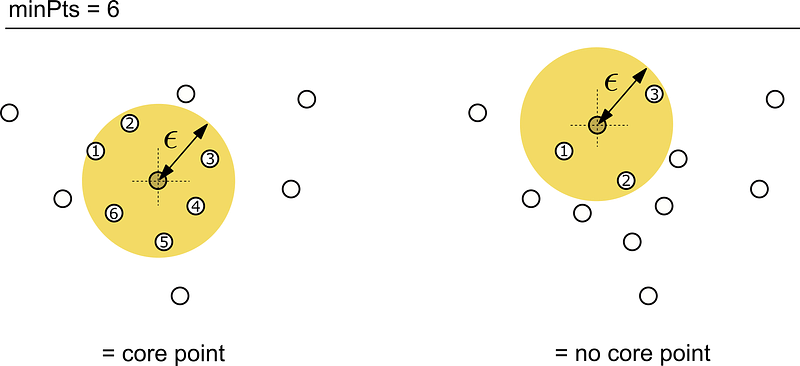
Density-reachable objects q are objects that do not reach this density value, but are directly reachable from a core objects. Data points to which none of these properties apply are called noise points and thus do not belong to the cluster. [Bre00][Zim][Int96][Kir02]

The following figure shows the step-by-step identification of core, densitiy-reachable and noise points.

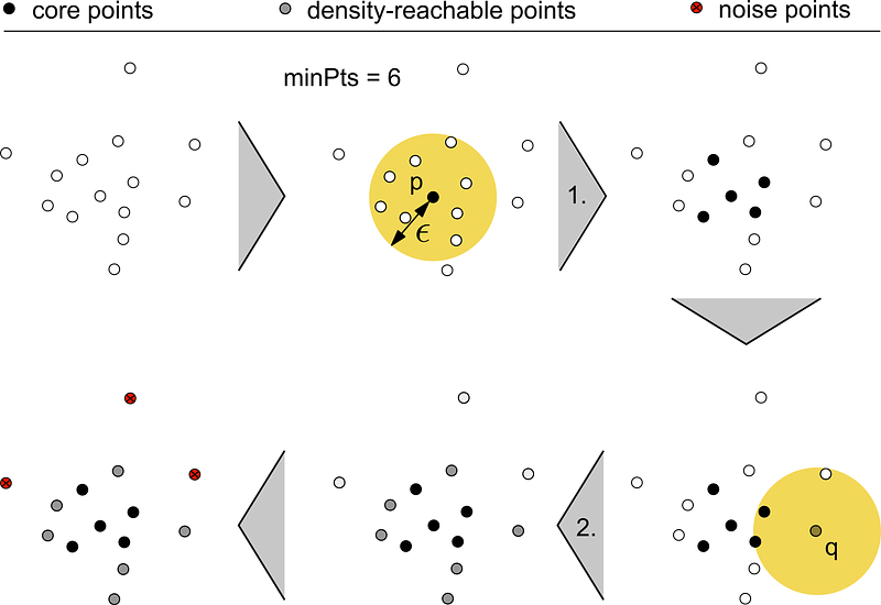
1. Identification of all core objects, which reach at least minPts = 6 in a distance ϵ.
2. Identification of the density-reachable points, which reach at least one core object in a distance of ϵ.

Instances that have not been identified as a core object or density-reachable objects up to this point represent noise points. These noise points represent the outliers or anomalous data points found.

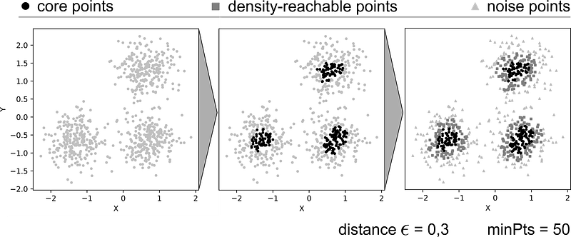
The following figure shows the classification of a more realistic dataset.

The LOF (Local Outlier Factor) algorithm adopts parts of the approach of the DBSCAN. The LOF additionally introduces the notion of reachability distance. The so-called k -distance is defined by the distance of an object to its k-nearest neighbor. [Kir02]

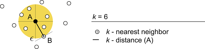
The reachability distance is defined by either the direct distance between objects A and B or the k-distance of object B. Objects within the distance k-distance are evaluated as equidistant, resulting in a more stable result.

Since it is possible for multiple objects to have the same distance, the set of values reachable in the k-distance may contain more than k objects. This set of neighbors is denoted as N_k(A). [Als10][Sch14]

The local reachability density (lrd) of an object A is calculated as follows:

Thus, the density is the reciprocal of the average reachability distance of object A from its neighbors.

This local reachability density is then compared with that of the neighboring instances [Bre00]:

A LOF_k(A) value of 1 indicates that the object A under consideration is comparable to its neighbors, i.e. it is not an outlier. Values below one, represent a higher density to the neighboring objects and thus an Inlier. Outliers are described by a value above one. In this case, the density is below that of the neighboring instances, which indicates an outlier.

One-Class Support Vector Machine

The Support Vector Machine (SVM) concept maps low-dimensional data to a new, higher-dimensional feature space. The subsequent learning process is performed on the transformed data. In this space, the data can be more easily separated and classified. [Kun04]

In the so-called linear separation (also linear classification), the data are divided into two groups by a linear line or plane, the so-called hyperplane [Kun04]. First introduced by Vapnik in 1963, linear classifiers are so called when the separation of the d-dimensional dataset is done by a (d-1)-dimensional hyperplane. [Jør08][Cor95]

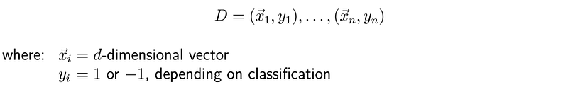
The so-called maximum-margin hyperplane (MMH) is sought, i.e. the hyperplane for which the distance to the nearest points with y_i=1 and y_i = -1is maximum. The hyperplane is defined as:

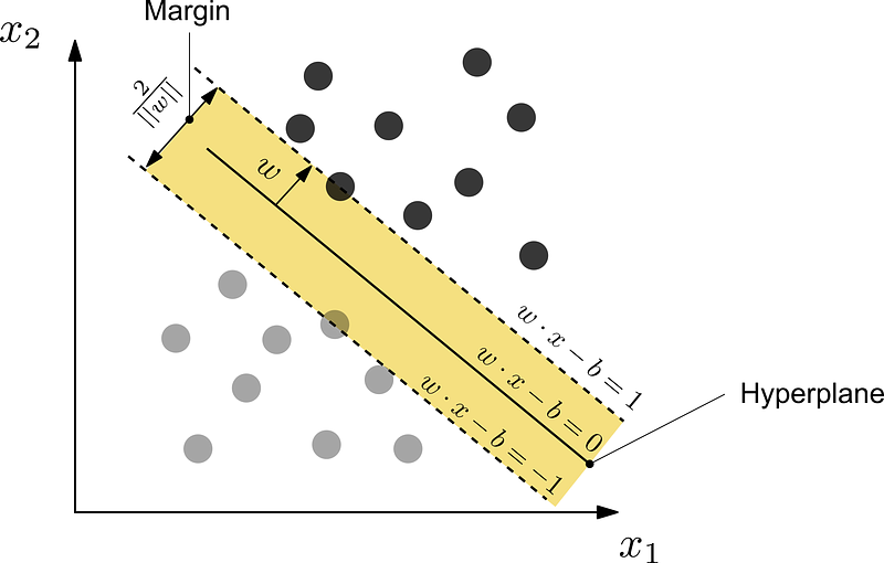
In most cases, the data cannot be separated by simple linear classification. This is where the Non-Linear Classifiers based on kernel functions are used, which allows the algorithm to find the MMH in a transformed, higher-dimensional feature space. The figure below shows a dataset that is not separable by a simple linear separator. In the example, the data are separated by a simple polynomial kernel (z = x 2 + y2 ) into a d + 1-dimensional feature space, in which the separation by a linear plane is possible.

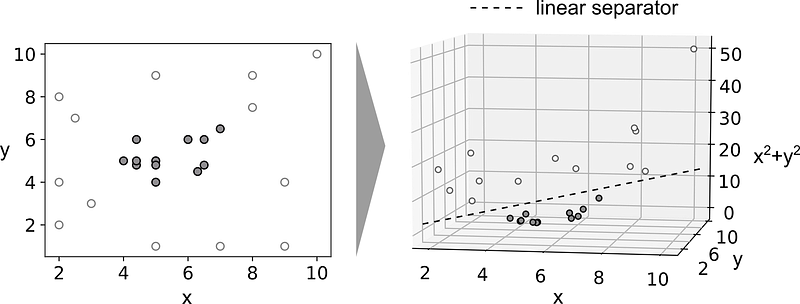
One-Class Classification

Schölkopf [Sch01] transfers the SVM methodology to a classification problem with only one class. [Bou14][Man01] Schölkopf’s approach sets a hyperplane in such a way that the distance ρ between the dataset and the origin is maximal [Tax01].

For this purpose, an algorithm was developed which returns a function f that takes the value +1 (range of normal instances) in a range that is as small as possible and in which the majority of the data points of the training dataset are included. The strategy transfers the initial data through a kernel k(x, y) into a higher-dimensional feature space. In this space, the dataset is separated from the origin in such a way that the distance ρ becomes maximum.

In addition to the Schölkopf method, the Tax and Duin method is often used. Here, the hyperplane does not take a planar form, but encloses the dataset with a sphere [Bou14].

You will find a more detailed explanation of how the One-Class SMV works in the sources used.

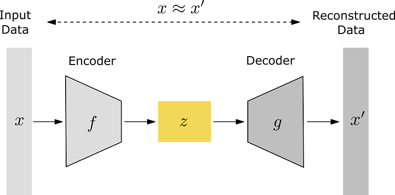
Autoencoder

Autoencoders are neural networks (NN) which are used to learn efficient data codings. [Kra91] They reconstruct the input signal through several hidden layers. The dimensions of the code are thereby restricted, forcing a dimensional reduction and enabling the identification of patterns.

An autoencoder comprises an encoder and a decoder. The encoder transforms the input into a coding by ignoring signal “noise”. The decoder transforms this new representation (coding) into the original form. Similar to dimensionality reduction, the autoencoder aims to replicate the input dataset as closely as possible.

Since the autoencoder is limited in its execution, forcing it to learn the features of the data that have the greatest impact on it. The goal is low-dimensional coding of high-dimensional data by recognizing structures and patterns in the data. Thus, the autoencoder searches for an encoder function f and a decoder function g that, after applying f to any element x of the d-dimensional input space X ⊂ R^d and then applying g to the resulting element z, yields the output element x as accurately as possible. [Saa18][Pie12]

Thus the autoencoder learns and replicates the most important features or in other words, the most frequently observed characteristics. Since “normal” data usually make up a much higher proportion of the training dataset, they are replicated very well. Rarely occurring “anomalous” data, on the other hand, are not replicated or not replicated sufficiently well. By simply comparing input data and reconstructed data, outliers can be identified. [An15]

Time Series Analysis

Data that are recorded sequentially over time are called time series [Bas07][Dei18].

If only one observation is assigned to each point in time (n = 1), we speak of univariate time series; if n > 1, we speak of multivariate time series. Time series analyses are of significant importance in areas of economics, stock trading and in the control of intelligent power grids [Mah16]. Since production processes are also characterized by cyclical processes, time series analysis is increasingly finding applications in manufacturing [Bas07][Keo06][Keo02]. Predicting time series provides important information for decision-making.

Regression methods model the relationship between the target variable y and several independent variables x1, x2, . . . , x_n. The value of the independent variable is not influenced by other features. [Bac06] Time Series Analysis, on the other hand, is limited to one independent variable x, the time, and is interested in predicting future target values. This is done by analyzing past data. Most methods aim to identify different signal components:

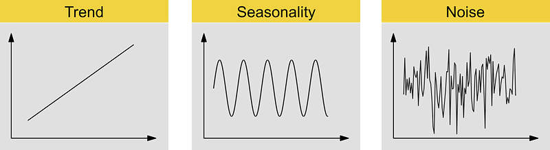
These components are used to predict the output signal without noise data. Instances or signal sections in the history are subsequently declared as Outlier/Anomaly if the deviation between predicted value and recorded signal exceeds a defined threshold.

Summary

Hope I could give you an overview of different techniques used to detect anomalies. Basically, the field of anomaly detection is not limited to specific algorithms. The approaches listed above are only used particularly often and should give you an understanding of some basic principles.

For your own use case, however, you should not feel limited by these. You should consider any statistical approach that allows you to distinguish between normal and anomalous instances.

If you found the article helpful, you can also find a similar article on concepts and algorithms used for Regression:

If you are not yet a Medium Premium member and plan to be, you can support me by signing up via the following referral link:

https://dmnkplzr.medium.com/membership

Thank you for reading!

References

[Als10] Alshawabkeh, M.; Jang, B.; Kaeli, D. Accelerating the local outlier factor algorithm on a GPU for intrusion detection systems. 2010.

[An15] An, Jinwon; Cho, Sungzoon: Variational Autoencoder based Anomaly Detection using Reconstruction Probability. 2015. [Bac06] Backhaus, K. Multivariate Analysemethoden: Eine anwendungsorientierte Einführung. 2006.

[Bas07] Basu, S.; Meckesheimer, M. Automatic outlier detection for time series: an application to sensor data. 2007.

[Bou14] Bounsiar, A.; Madden, M. G., Herausgeber. One-Class Support Vector Machines. 2014.

[Bre00] Breunig, M.; Kriegel, H.-P.; Ng, Raymond,Sander, Jörg. LOF: Identifying Density-Based Local Outliers. 2000.

[Cha09a] Chandola, V.; Banerjee, A.; Kumar, V. Anomaly detection. 2009. [Cor95] Cortes, C.; Vapnik, V. Support-Vector Networks. 1995.

[Dei18] Deistler, M.; Scherrer, W. Zeitreihen und stationäre Prozesse. 2018.

[Ert16] Ertel, W. Grundkurs Künstliche Intelligenz: Eine praxisorientierte Einführung. 2016.

[Eur10] Factoriers of the Future PPP, 2010. URL https://op.europa.eu/de/publication-detail/-/publication/0f4eaca5-05f1-4532-937e-f504441f73e0

[Fah16] Fahrmeir, L.; Heumann, C.; Künstler, R. Statistik: Der Weg zur Datenanalyse. 2016.

[Fer03] Fernuni Hagen. Gemeinsame Wahrscheinlichkeitsverteilung. 2003.

[Gue15] Guerbai, Y.; Chibani Y.; Hadjadji, Bilal. The effective use of the one-class SVM classifier for handwritten signature verification based on writer-independent parameters. 2015.

[Har18] Hariri, S.; Kind, M. C. Isolation Forest for Anomaly Detection. 2018. [Has09] Hastie, T.; Tibshirani, R.; Friedman, J. The Elements of Statistical Learning: Data Mining, Inference, and Prediction. 2009.

[Haz02] Hazewinkel, M. Encyclopaedia of mathematics. 2002.

[Hod04] Hodge, V. J.; Austin, J. A Survey of Outlier Detection Methodologies. 2004.

[Hot04] Hotho, A. Clustern mit Hintergrundwissen. 2004.

[Int96] Proceedings / Second International Conference on Knowledge Discovery & Data Mining. 1996.

[Jør08] Jørgensen, S. E. Encyclopedia of ecology. 2008.

[Keo02] Keogh, E.; Lonardi, S.; Chiu, B. Y.-c. Finding Surprising Patterns in a Time Series Database in Linear Time and Space. 2002.

[Keo06] Keogh, E.; Lin, J.; Lee, S.-H.; van Herle, H. Finding the most unusual time series subsequence: algorithms and applications. 2006.

[Kir02] Kirgel, H.-P. Hauptseminar KDD: Clustering. 2002. URL https://www.dbs.ifi.lmu.de/Lehre/Hauptseminar/SS02/KDD02/Clustering-Peer.pdf

[Koi18] Koizumi, Y.; Saito, S.; Uematsu, H.; Kawachi, Y.; Harada, N. Unsupervised Detection of Anomalous Sound Based on Deep Learning and the Neyman–Pearson Lemma. 2018.

[Kra91] Kramer, Mark A. “Nonlinear principal component analysis using autoassociative neural networks” (PDF). 1991.

[Kun04] Kunze, K. Hauptseminar Machine Learning: Support Vector Machines. 2004. URL http://campar.in.tum.de/twiki/pub/Far/MachineLearningWiSe2003/kunze_ausarbeitung.pdf

[Liu12] Liu, F. T.; Ting, K. M.; Zhou, Z.-H. Isolation-Based Anomaly Detection. ACM Transactions on Knowledge Discovery from Data, 2012. https://cs.nju.edu.cn/zhouzh/zhouzh.files/publication/tkdd11.pdf

[Mah16] Mahalakshmi, G.; Sridevi, S.; Rajaram, S. A Survey on Forecasting of Time Series Data, 2016.

[Man01] Manevitz, L. M.; Yoused, M. One-Class SVMs for Document Classifcation. 2001.

[Ott18] Otto, T. Anomalie-Erkennung mit Machine Learning. 2018.

[Pat18] Patel, A. A. Hands-On Unsupervised Learning Using Python. O’Reilly Media, Inc, 2018.

[Pie12] Pierre Baldi. Autoencoders, Unsupervised Learning, and Deep Architectures. Proceedings of ICML Workshop on Unsupervised and Transfer Learning, 2012.

[Ras18] Raschka, S.; Mirjalili, V. Machine Learning mit Python und Scikit-Learn und TensorFlow: Das umfassende Praxis-Handbuch für Data Science, 2018.

[Saa18] Saalmann, E. Einführung in Autoencoder und Convolutional Neural Networks. 2018. URL https://dbs.uni-leipzig.de/file/Saalmann_Ausarbeitung.pdf

[Sch01] Schölkopf, B.; Platt, J.; Shawe-Taylor, J.; Smola, A.; C. Williamson, R. Estimating Support of a High-Dimensional Distribution. Neural Computation

[Sch14] Schubert, E.; Zimek, A.; Kriegel, H.-P. Local outlier detection reconsidered: A generalized view on locality with applications to spatial, video, and network outlier detection. Data Mining and Knowledge Discovery, 28, 2014.

[Sci19a] 2.6. Covariance estimation — scikit-learn 0.21.1 documentation, 2019.

[Sci19b] ScikitLearn. 2.7. Novelty and Outlier Detection — scikit-learn 0.21.1 documentation, 2019. URL https://scikit-learn.org/stable/modules/outlier_detection.html

[Sha13] Sharafi, A. Knowledge Discovery in Databases. Springer Fachmedien Wiesbaden, Wiesbaden, 2013.

[Spe14] Probabilistisches Verfahren, 04.12.2014. https://www.spektrum.de/ lexikon/geographie/probabilistisches-verfahren/6232ren/6232

[Tax01] Tax, D. M. J. One-Class Classification. 2001.

[Vie19] Vieira, R. Introduction to Isolation Forests · Rui Vieira, 2019. URL https://ruivieira.github.io/introduction-to-isolation-forests.html

[Win15] Windmann, S.; Maier, A.; Niggemann, O.; Frey, C.; Bernardi, A.; Gu, Y.; Pfrommer, H.; Steckel, T.; Krüger, M.; Kraus, R. Big Data Analysis of Manufacturing Processes. Journal of Physics: Conference Series, 2015.

[Yan16] Yang, Jinhong; Deng, Tingquan. An Adaptive Weighted One-Class SVM for Robust Outlier Detection. Proceedings of the 2015 Chinese Intelligent Systems Conference. 2016

[Zim] Zimek, A. Clustering Teil 2. URL https://www.dbs.ifi.lmu.de/Lehre/KDD/SS14/skript/KDD-3-Clustering-2.pdf

[Zim18] Zimek, A.; Schubert, E. Outlier Detection, 2018.