Free AI web copilot to create summaries, insights and extended knowledge, download it at here
2360
Abstract
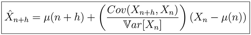
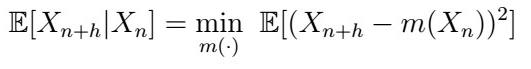
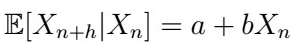
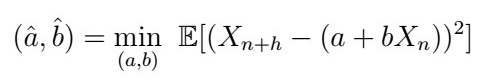
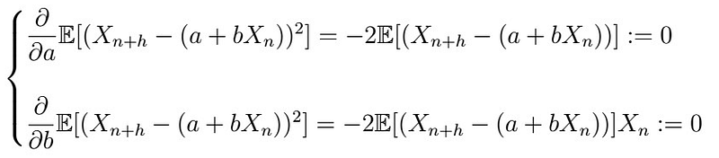
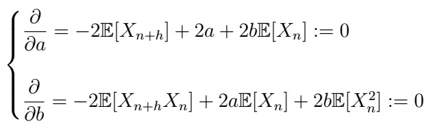
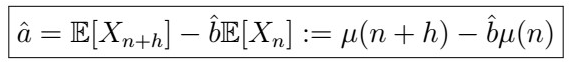
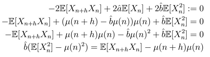
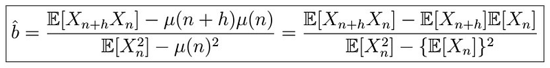
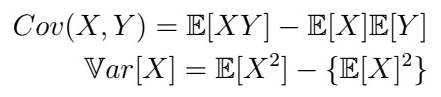
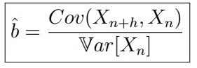
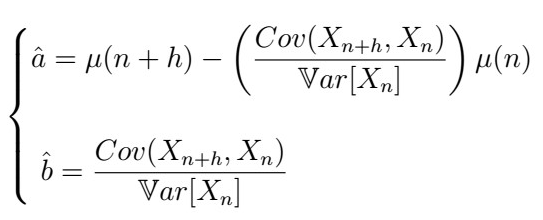
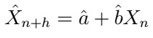
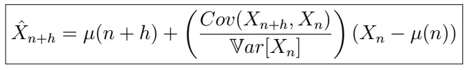
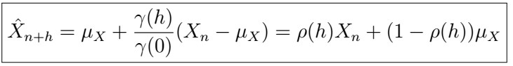
gcaption></figcaption></figure><p id="e978">so now we can solve for a, say. You can verify that the solution is given by</p><figure id="df13"><img src="https://cdn-images-1.readmedium.com/v2/resize:fit:800/1*WOKCeS8qdJyiKk2u0vBq4Q.png"><figcaption></figcaption></figure><p id="7232">where we used “\mu” to represent the expectation as a function of the inner lag. Next, plugging back and solving for b, we obtain</p><figure id="e915"><img src="https://cdn-images-1.readmedium.com/v2/resize:fit:800/1*CW8phDH_atbzuqN8R347xw.png"><figcaption></figcaption></figure><p id="fbef">so that</p><figure id="920d"><img src="https://cdn-images-1.readmedium.com/v2/resize:fit:800/1*xEsge9iqEmg85xA1Ep9lAQ.png"><figcaption></figcaption></figure><p id="520e">Does this look familiar? Recall that</p><figure id="643f"><img src="https://cdn-images-1.readmedium.com/v2/resize:fit:800/1*-O7hh7CDc0GoV0zmAUAy9g.png"><figcaption></figcaption></figure><p id="3e98">So that the expression above becomes</p><figure id="d7ec"><img src="https://cdn-images-1.readmedium.com/v2/resize:fit:800/1*4yqJDeTtffxnDhdWEH9-vQ.png"><figcaption></figcaption></figure><p id="726c">Now, plugging this back once more into “a”, gives</p><figure id="1f83"><img src="https://cdn-images-1.readmedium.com/v2/resize:fit:800/1*i0Aqeoxs5Q7ZmTCv6dJrKw.png"><figcaption></figcaption></figure><p id="dde9">Therefore, if we denote our B.L.P as</p><figure id="44a8"><img src="https://cdn-images-1.readmedium.com/v2/resize:fit:800/1*RjhhFGfhXrHB9U9Zq1LaGQ.png"><figcaption></figcaption></figure><p id="8fec">we see that</p><figure id="f9eb"><img src="https://cdn-images-1.readmedium.com/v2/resize:fit:800/1*5tPUgiSUiw8vaPsvOoyzRQ.png"><figcaption></figcaption></figure><p id="04cc">and this is precisely the formula you saw at the beginning! How is this useful? Suppose that you have, in addition, a <b>stationary series</b>. Then the BLP is given by</p><figure id="a080"><img src="https://cdn-images-1.readmedium.com/v2/resize:fit:800/1*KEtC_AijpGNjZUgMq-LXWQ.png"><figcaption></figcaption></figure><p id="8a0a">and if the ACF is between 0 and 1, we have a weighted average between the <b>most recent observation</b> and the <b>overall trend. </b>Isn’t that fascinating?! Note that we dropped the argument for the mean since a stationary series mean is constant, and further, the covariance and variance just beco
Options
me the autocovariance function of the series.</p><h2 id="0f9a">Next time</h2><p id="1419">Next time, we will start studying Linear Processes. which will be extremely useful when dealing with ARMA , ARIMA and other models. Stay tuned, and happy learning!</p><h2 id="f9b9">Last time</h2><p id="455b"><a href="https://medium.com/@hair.parra/a-complete-introduction-to-time-series-analysis-with-r-tests-for-stationarity-prediction-1-a78c1cf16676">Prediction 1 → Best Linear Predictor I</a></p><div id="f1a2" class="link-block">
<a href="https://medium.com/@hair.parra/a-complete-introduction-to-time-series-analysis-with-r-tests-for-stationarity-prediction-1-a78c1cf16676">
<div>
<div>
<h2>A Complete Introduction To Time Series Analysis (with R):: Tests for Stationarity:: Prediction 1 →…</h2>
<div><h3>We’ve come a long way: from studying models to study time series, stationary processes such as the MA(1) and AR(1)…</h3></div>
<div><p>medium.com</p></div>
</div>
<div>
<div style="background-image: url(https://miro.readmedium.com/v2/resize:fit:320/1*UlrclDUaBEPQdFz42-Csnw.png)"></div>
</div>
</div>
</a>
</div><h2 id="54b0">Main page</h2><div id="dddc" class="link-block">
<a href="https://readmedium.com/a-complete-introduction-to-time-series-analysis-with-r-9882f2d44c9d">
<div>
<div>
<h2>A Complete Introduction To Time Series Analysis (with R)</h2>
<div><h3>During these times of the Covid19 pandemic, you have perhaps heard about the collaborative efforts to predict new…</h3></div>
<div><p>medium.com</p></div>
</div>
<div>
<div style="background-image: url(https://miro.readmedium.com/v2/resize:fit:320/1*TL2PeOANEN4zG0_OqoHptQ.jpeg)"></div>
</div>
</div>
</a>
</div><h2 id="653d">Follow me at</h2><ol><li><a href="https://www.linkedin.com/in/hair-parra-526ba19b/">https://www.linkedin.com/in/hair-parra-526ba19b/</a></li><li><a href="https://github.com/JairParra">https://github.com/JairParra</a></li><li><a href="https://medium.com/@hair.parra">https://medium.com/@hair.parra</a></li></ol></article></body>