Data Analysis

A complete Data Analysis workflow in Python and scikit-learn

A ready-to-run code including preprocessing, parameters tuning and model running and evaluation.

In this short tutorial I illustrate a complete data analysis process which exploits the scikit-learn Python library. The process includes

• preprocessing, which includes features selection, normalization and balancing
• model selection with parameters tuning
• model evaluation

The code of this tutorial can be downloaded from my Github Repository.

Load Dataset

Firstly, I load the dataset through the Python pandas library. I exploit the heart.csv dataset, provided by the Kaggle repository.

import pandas as pd

df = pd.read_csv('source/heart.csv')
df.head()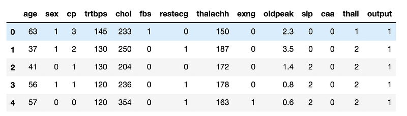

I calculate the number of records and the number of columns in the dataset:

df.shape

which gives the following output:

(303, 14)

Features selection

Now, I split the columns of the dataset in input (X) and output (Y). I use all the columns but output as input features.

features = []
for column in df.columns:
    if column != 'output':
        features.append(column)
X = df[features]
Y = df['output']

In order to select the minimum set of input features, I calculate the Pearson correlation coefficient among features, through corr() function, provided by a pandas dataframe.

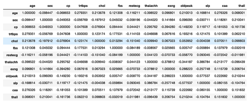
I note that all the features have a low correlation, thus I can keep all of them as input features.

Data Normalization

Data Normalization scales all the features in the same interval. I exploit the MinMaxScaler() provided by the scikit-learn library. I dealt with Data Normalization in scikit-learn in my previous article, while I this article I described the general process of Data Normalization without scikit-learn.

X.describe()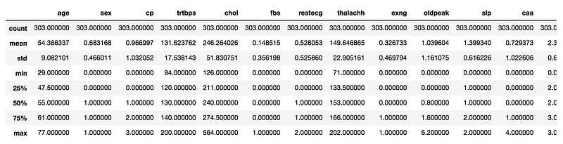

Looking at the minimum and maximum value for each feature, I note that there are many features out the range [0,1], thus I need to scale them.

For each input feature I calculate the MinMaxScaler() and I store the result in the same X column. The MinMaxScaler() must be fitted firstly through the fit() function and then can be applied for a transformation through the transform() function. Note that I must reshape every feature in the format (-1,1) in order to be passed as input parameter of the scaler. For example, Reshape(-1,1) transforms the array [0,1,2,3,5] into [[0],[1],[2],[3],[5]].

from sklearn.preprocessing import MinMaxScaler

for column in X.columns:
    feature = np.array(X[column]).reshape(-1,1)
    scaler = MinMaxScaler()
    scaler.fit(feature)
    feature_scaled = scaler.transform(feature)
    X[column] = feature_scaled.reshape(1,-1)[0]

Split the dataset in Training and Test

Now I split the dataset into two parts: training and testset. The test set size is 20% of the whole dataset. I exploit the scikit-learn function train_test_split(). I will use the training set to train the model and the testset to test the performance of the model.

import numpy as np
from sklearn.model_selection import train_test_split

X_train, X_test, y_train, y_test = train_test_split( X, Y, test_size=0.20, random_state=42)

Balancing

I check whether the dataset is balanced or not, i.e. if the output classes in the training set are equally represented. I can use the value_counts() function to calculate the number of records in each output class.

y_train.value_counts()

which gives the following output:

1    133
0    109

The output classes are not balanced, thus I can balance it. I can exploit the imblearn library, to perform balancing. I try both oversampling the minority class and undersampling the majority class. More details related to the Imbalanced Learn library can be found here. Firstly, I perform over sampling through the RandomOverSampler(). I create the model and then I fit with the training set. The fit_resample() function returns the balanced training set.

from imblearn.over_sampling import RandomOverSampler
over_sampler = RandomOverSampler(random_state=42)
X_bal_over, y_bal_over = over_sampler.fit_resample(X_train, y_train)

I calculate the number of records in each class through the value_counts() function and I note that now the dataset is balanced.

y_bal_over.value_counts()

which gives the following output:

1    133
0    133

Secondly, I perform under sampling through the RandomUnderSampler() model.

from imblearn.under_sampling import RandomUnderSampler

under_sampler = RandomUnderSampler(random_state=42)
X_bal_under, y_bal_under = under_sampler.fit_resample(X_train, y_train)

Model Selection and Training

Now, I’m ready to train the model. I choose a KNeighborsClassifier and firstly I train it with imbalanced data. I exploit the fit() function to train the model and then thepredict_proba() function to predict the values of the test set.

from sklearn.neighbors import KNeighborsClassifier

model = KNeighborsClassifier(n_neighbors=3)
model.fit(X_train, y_train)
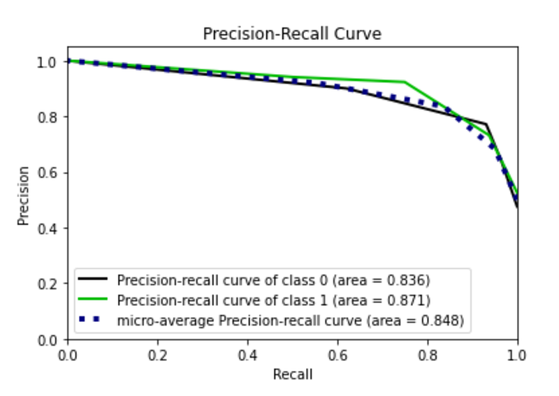
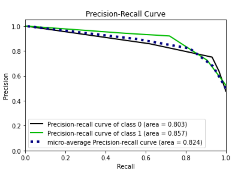
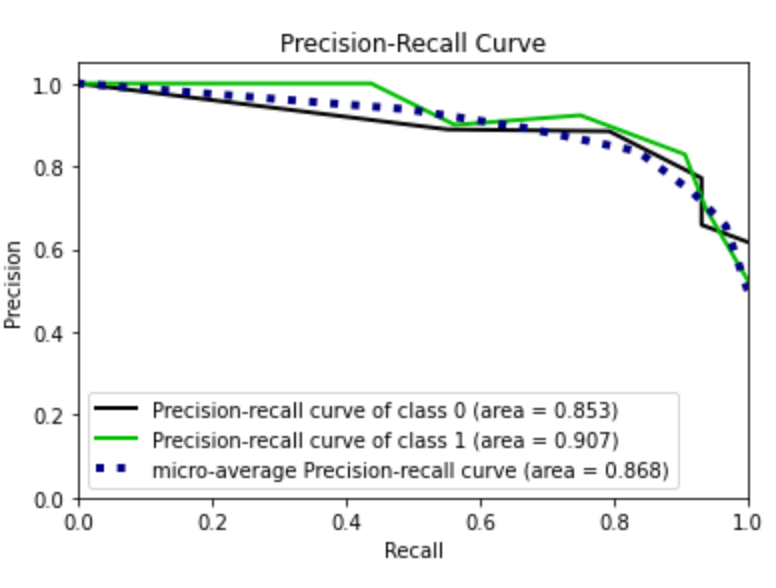
y_score = model.predict_proba(X_test)

I calculate the performance of the model. In particular, I calculate the roc_curve() and the precision_recall() and then I plot them. I exploit the scikitplot library to plot curves.

From the plot I note that there is a roc curve for each class. With respect to the precision recall curve, the class 1 works better than class 0, probably because it is represented by a greater number of samples.

import matplotlib.pyplot as plt
from sklearn.metrics import roc_curve
from scikitplot.metrics import plot_roc,auc
from scikitplot.metrics import plot_precision_recall

fpr0, tpr0, thresholds = roc_curve(y_test, y_score[:, 1])

# Plot metrics 
plot_roc(y_test, y_score)
plt.show()
    
plot_precision_recall(y_test, y_score)
plt.show()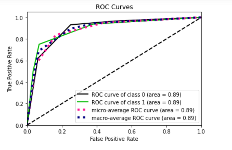

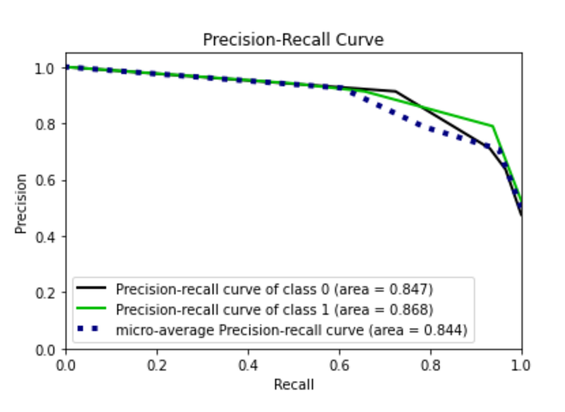
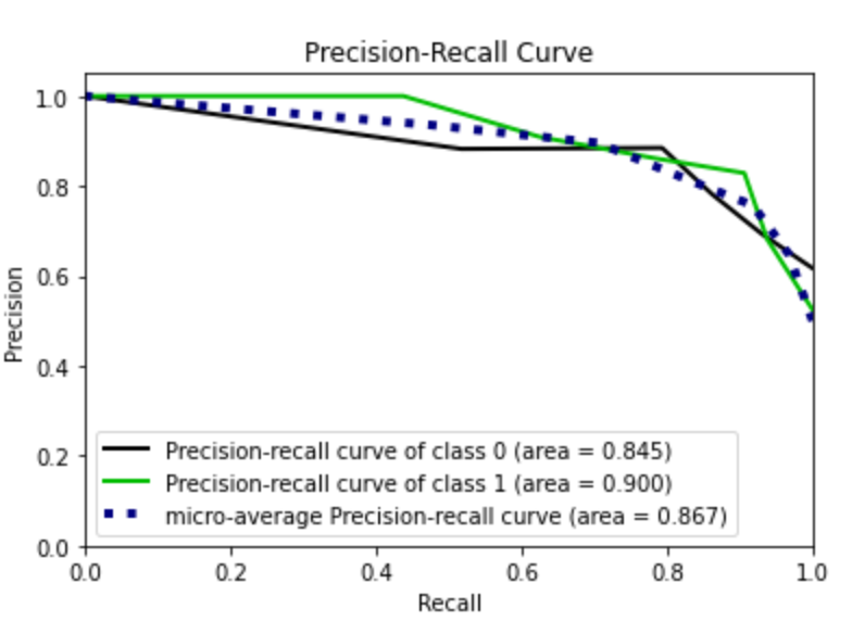
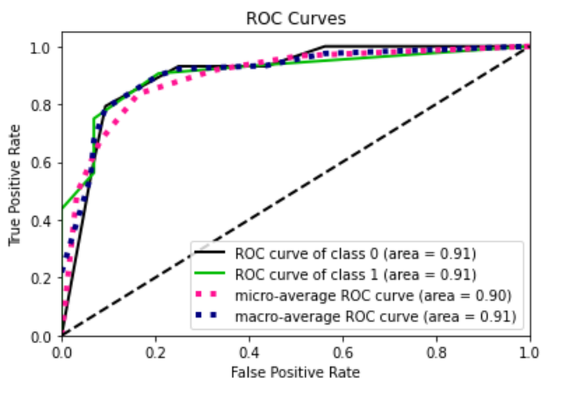
Now, I recalculate the same things with oversampling balancing. I note that the precision recall curve of class 0 increases, while that of class 1 decreases.

model = KNeighborsClassifier(n_neighbors=3)
model.fit(X_bal_over, y_bal_over)
y_score = model.predict_proba(X_test)
fpr0, tpr0, thresholds = roc_curve(y_test, y_score[:, 1])

# Plot metrics 
plot_roc(y_test, y_score)
plt.show()
    
plot_precision_recall(y_test, y_score)
plt.show()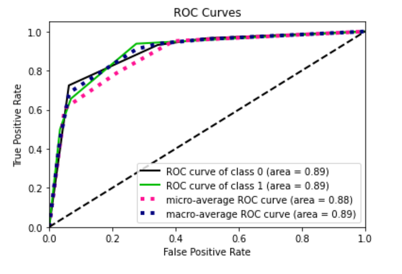

Finally, I train the model through under sampled data and I note a general deterioration of the performance.

model = KNeighborsClassifier(n_neighbors=3)
model.fit(X_bal_under, y_bal_under)
y_score = model.predict_proba(X_test)
fpr0, tpr0, thresholds = roc_curve(y_test, y_score[:, 1])

# Plot metrics 
plot_roc(y_test, y_score)
plt.show()
    
plot_precision_recall(y_test, y_score)
plt.show()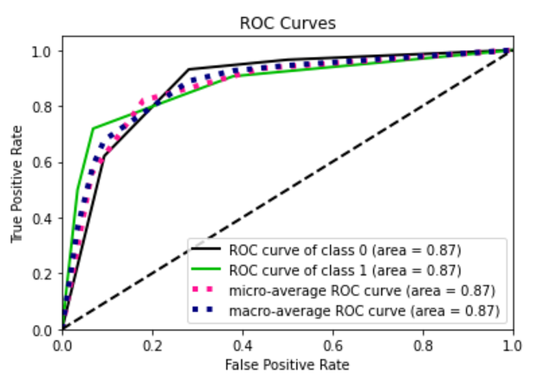

Parameters Tuning

In the last part of this tutorial, I try to improve the performance of the model by searching for best parameters for my model. I exploit the GridSearchCV mechanism provided by the scikit-learn library. I select a range of values for each parameter to be tested and I put them in the param_grid variable. I create a GridSearchCV() object, I fit with the training set and then I retrieve the best estimator, contained in the best_estimator_ variable.

from sklearn.model_selection import GridSearchCV

model = KNeighborsClassifier()

param_grid = {
   'n_neighbors': np.arange(2,8),
   'algorithm' : ['auto', 'ball_tree', 'kd_tree', 'brute'],
    'metric' : ['euclidean','manhattan','chebyshev','minkowski']
}

grid = GridSearchCV(model, param_grid = param_grid)
grid.fit(X_train, y_train)

best_estimator = grid.best_estimator_

I exploit the best estimator as model for my predictions and I calculate the performance of the algorithm.

best_estimator.fit(X_train, y_train)
y_score = best_estimator.predict_proba(X_test)
fpr0, tpr0, thresholds = roc_curve(y_test, y_score[:, 1])

# Plot metrics 
plot_roc(y_test, y_score)
plt.show()
    
plot_precision_recall(y_test, y_score)
plt.show()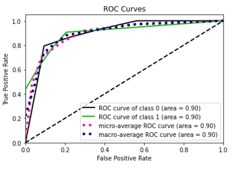

I note that the roc curve has improved. I try now with the over sampled training set. I omit the code because it is the same as before. In this case I obtain the best performance.

Summary

In this tutorial I have illustrated the full workflow to build a good model for data analysis. The workflow includes:

• data preprocessing, with features selection and balancing
• model selection and parameters tuning with Grid Search with Cross Validation
• model evaluation, through the ROC curve and the Precision Recall curve.

In this tutorial I have not dealt with Outliers Detection. If you want to learn something about this aspect, you can give a look to my previous article.

If you wanted to be updated on my research and other activities, you can follow me on Twitter, Youtube and and Github.

Related Articles

New to Medium? You can subscribe for few dollars per month and unlock unlimited articles — click here.