A 10-Minute Space Battle Movie in 1000 Lines of Code: Part 1. The Simulation

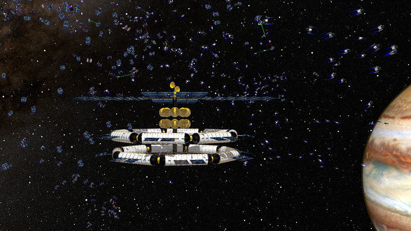
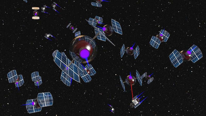
500 spaceships, a rotating space station, a planet, stars, lasers, and explosions. No video or 3D editing, just code.

Introduction

I am a big fan of space battles in movies. They are fun to watch. Yet mostly, they are relatively short, with only a few blurry spaceships. So I decided to create my own.

Can I create a space battle? Probably. I would need to learn how to create special effects using some software I don’t have.

As a programmer, I know Python. And I used to play with a 3D raytracer. Can I combine these skills to create a 10-minute film with a fast, dynamic space battle and stunning visuals?

What are the parts needed to create such a film?

A Simulation. I want to model the movement of the spaceships using a simulation system. They should be able to avoid crashing into each other or the space station. They attack opponents and blow them up.

3D renderer. The simulation delivers the trajectory of the spaceships. A 3-dimensional image of the spaceships and their surroundings is required to create a film. A renderer accepts a scene description file as input and outputs a single image.

Sound effects. There is no sound in space. And lasers are silent on earth, too. Still, every space movie uses sound effects because they significantly improve the experience.

Film editing. I want different camera angles. Some follow the spaceships, and some provide an overview or a detail from one static location. And finally, everything needs to be combined into a film I can upload and share.

What is not necessary is a computer mouse. Everything I explain here can be done in a simple text editor. Why would I do that? Because it is fascinating that this is even possible. This leads to a

Disclaimer

The film is based on the output of a simulation. I am not interested in creating the best film possible. I want to model the behavior of spaceships. I do not want to draw a path they fly in a way it looks good in the film. The spaceships are guided by the laws of physics and simple rules.

Likewise, I am not interested in painting textures for the objects to look good. I define materials and surface properties, and the image results from the physics of light applied to these objects.

The whole point of this article series is to show that the emerging result can be spectacular if you take a really simple simulation and some small object definitions and cleverly combine them.

Integrated VFX solutions support simulations and rendering pipelines in one package or as plugins. If you have to create a movie, that might be the better approach.

The Simulation

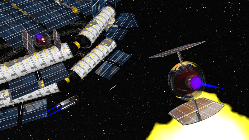
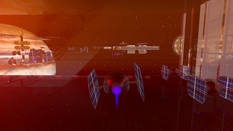
This is a space battle simulation. Two types of spaceships fight each other. They start at random locations outside the field of view and then fly toward each other.

Once they spot a spaceship of the other type, they chase it and try to attack it. Their weapon is a laser. They can’t fire constantly; some recharging is required in between shots. A spaceship that is hit by lasers too often explodes.

The rules that guide the spaceships are simple. Nevertheless, exciting flight maneuvers happen, and fascinating patterns emerge.

Internally, 500 spaceships have a position and a velocity each. Time is modeled in discrete timesteps, incremented in a main loop.

There are particle-based Lagrangian and grid-based Eulerian simulations. For both types, typically, vectorized programming is a performant solution. All positions and velocities, or grid cells, respectively, are stored in an array and updated simultaneously.

The example simulation used here is a dynamic Lagrangian simulation. The position and trajectory of elements are calculated individually as they move through space and time. What makes it more complex is the fact that elements are added and deleted dynamically. And the behavior of the elements is more sophisticated than with simple physics-based particles.

Therefore, an object-oriented approach has been chosen here. It is slower to run, but the program structure is cleaner. An earlier article presents a speed comparison of different techniques and programming languages [1].

3 Dimensions

I wrote an article about such a simulation before[2]. This time, the simulation is 3-dimensional. This is similar. All that is needed to add a dimension is to store one more value per vector and update all formulas.

I used NumPy as a library for storing vectors and performing calculations. The benefit is that geometrical operations like vector length normalization are already defined. The code is short and readable by anyone familiar with scientific libraries. The drawback, however, is that NumPy is not optimized for short vectors like the one used here. The simulation is not fast — but readability is more important in this case. A good discussion on this issue can be found here.

Components

To update a spaceship’s position, we need to know its velocity vector (Δx/Δy/Δz). Every spaceship has a desired velocity. This is how fast and in which direction the agent wants to move. The actual velocity of a spaceship is limited by its maximal speed and other constraints, such as the presence of other spaceships.

It makes sense to think of forces f that push or pull the spaceship in a certain direction. Then, we can use the formula

to calculate the acceleration a of each spaceship. In this simulation, all spaceships have the same mass m of 1. Four forces are used:

• The social force dictates near-distance interactions between spaceships. It is similar to the one described in the paper Social Force Model for Pedestrian Dynamics[3].
• The force that points to the next enemy spaceship to follow and attack it. This force is voluntary for the spaceship; it represents its free will to move.
• A force field that defines a no-fly zone around other objects in the simulations, like the space station, for example. In theory, a spaceship could ignore such a constraint. Here, the forces from the fields are just added and become mandatory for the spaceship to observe.
• Finally, a force field pulls the spaceships back to the center of the simulation, analog to the no-fly zone field.

The social force

This is the most elemental of the forces here. It separates the spaceships from each other. As soon as two spaceships get too close to each other, a force vector in the opposite direction starts to grow.

The direction is away from the other spaceship. The length is based on a formula, as shown in the graph below.

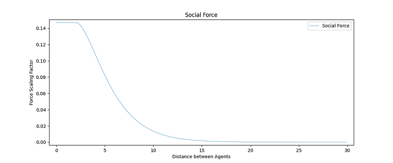
In the range of 15 down to 5 meters, the force slowly increases. This gradual force increase ensures that affected spaceships do not abruptly change their course. They steer slowly away from each other once they get too close.

force = np.array([0, 0, 0], dtype=np.float64)
for a in self.neighbors:
    distance = np.linalg.norm(self.position - a.position)

    if distance < 2:
        factor = 2 / np.exp(0.5 * 2)
    else:
        factor = distance / np.exp(0.5 * distance)

    force = force + factor * (self.position - a.position)

This iteration over all spaceships has the effect that the runtime of the simulation is O(n2). This is fine for a small number of spaceships, say up to 500, depending on your computer and patience.

For more spaceships, more sophisticated handling of spaceships is required. For example, a simple list of nearest neighbors can help a lot.

Follow the nearest enemy

This third force is quite simple. The spaceship needs to follow an enemy spaceship to attack it.

The force pulls in the direction of the associated enemy. This force is constant no matter how far away the enemy is.

direction = (self.target.position - self.position)
force = direction / np.linalg.norm(direction) 

The no-fly zone force

A large rotating space station floats near the center of the simulation. It is there for purely aesthetic reasons later in the 3-dimensional film. However, the spaceships must know its existence, so they avoid that area.

As with the social force above, this force needs to increase gradually the closer the spaceships get to the space station.

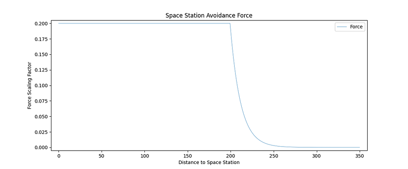
The formula is similar to the one of the social force. The advantage is that in this simulation, only one space station exists. In more complex scenarios, a list of objects to iterate over would be necessary.

station = np.array([0, 500, 40], dtype=np.float64)

direction = (self.position - station)
distance = np.linalg.norm(direction)

factor = min(0.2, np.exp(-(distance-180)/12))  # soft transition
direction = direction / distance

force = factor * direction

The center force

The force that directs the spaceships back to the center of the simulation is simple. It’s the squared distance to the center, so the farther away they are, the bigger the force becomes.

direction = (self.position)
distance = np.linalg.norm(direction)

factor = distance ** 2 / 1000000

force = factor * (-direction / distance)

Of course, this force is optional and purely for this film. In reality, spaceships should be free to fly wherever they want.

Updating all the forces and the velocity

In the update() method, all forces are added together. Each force has a different weight, which is used to fine-tune the dynamics of the simulation.

In each time step of the simulation, the forces are calculated. This vector is also the acceleration vector, as we assume all spaceships have the same mass. The forces are not real forces like gravity anyway; they model the behavior of someone steering the spaceship.

These forces are added to the velocity of the last timestep t-1 to calculate the velocity of the current timestep t:

According to this formula, in each timestep t, the spaceships would move forward one unit of v. However, a timestep represents one frame in the final film, which runs at 24 Hz or frames per second. An additional variable to control this timestep granularity Δt is required. It is traditionally called h in the code and is set to 0.2.

# target is dead, don't chase it further
if self.target and (self.target not in agents or not self.target.is_alive):
    self.target = None

# find and attack targets
self.find_target(agents, max_distance=100**2)
self.attack(systemtime, output_file, max_distance=500)  # was 350

# the neighbor cache is for faster access to agents nearby
if systemtime % 10 == 0:
    self.reset_neighbor_cache(agents, max_distance=10000)

# calculate the forces
f_social = self.calculate_force_social()
f_center = self.calculate_force_center()
f_nofly = self.calculate_force_nofly_zone()
f_target = self.calculate_force_target()

force = 0.2 * f_social + 0.4 * f_center + 0.1 * f_nofly + 0.4 *f_target

# update direction based on the forces 
# Leapfrog integration (https://en.wikipedia.org/wiki/Leapfrog_integration)
self.velocity = self.velocity + h * 0.5 * (self.force + force)
self.force = force

# slow down agent if it moves faster than its max velocity 
velocity = np.linalg.norm(self.velocity)
if velocity > (Agent.vmax * h):
    self.velocity = self.velocity / velocity * (Agent.vmax * h)

Apart from code to calculate the forces, this snippet also shows some logic to find enemies at the top. These methods are relatively technical and less entertaining. I will redirect you to the GitHub repository if you are interested.

Fighting

Once within range of an enemy, the spaceships want to fight them. In this simulation, there is no need to aim. The laser always fires in the direction of the target.

For the film, it is preferable to have individual shots fired at an enemy. Each of them will have its sound effect. For this, there is a firing probability. There is a certain (low) probability that the laser is actually fired in each time step.

distance = Agent.square_distance(self.position - self.target.position)

if distance < max_distance:
    if random.random() <= probability:  # shoot not too often, reloading or sth
        print(f"{systemtime}, Shot, {self.id}, {self.target.id}", file=output_file)
        self.target.hit(systemtime, output_file, damage=2.5)

Since the laser aims automatically, the spaceships will always hit their enemy once they fire. Each time, a certain amount of energy is deducted from the enemy spaceship. Once its energy levels reach 0, it explodes.

self.energy = self.energy - h * damage  # damage per shot

if self.energy < 0:
    if self.target:
        self.target.targeted -= 1

    self.is_alive = False
    print(f"{systemtime}, Explosion, {self.id}", file=output_file)

Both events have to be reported in the log file for later processing.

Main Loop Structure

Before I explain the main loop of the simulation, here is a quick word about the update dynamics.

If both positions and forces were updated in the same method, the updates would be calculated for each spaceship independently. This leads to the effect that one spaceship would calculate its forces based on neighbor positions that still need to be updated.

The update methods for positions and the rest are separated to solve this. First, all positions based on the last timestep’s velocities are calculated (move()). Then, using the forces, new velocities are computed (update()). These affect the spaceships in the next time step.

These update dynamics are called Gauss-Seidel and Jacobi, respectively. Jacobi is better for potential parallelization since positions can be updated independently.

Using standard Eulerian integration, the velocity is added to the position. Since the velocity is taken at the beginning of each timestep, it is only valid for a very short time (small values of Δt or h). After that, the acceleration changes the velocity.

To improve accuracy, a method called leapfrog integration can be used. Each position update is refined using a correction factor based on the acceleration.

And something similar happens in the update function above for the velocity v. It is based on an average of the last and current timestep’s force f:

(If these formulas are too complex, use simple Eulerian integration. I doubt that anyone spots the difference in the film!)

# update position based on velocity and a half step of the force (Leapfrog)
delta_position = h * self.velocity + (0.5 * self.force) * h ** 2

# slow down agent if it moves faster than its max velocity
delta_position_norm = np.linalg.norm(delta_position)
if delta_position_norm > (Agent.vmax * h):
    delta_position = delta_position / delta_position_norm * (Agent.vmax * h)

self.position = self.position + delta_position

message = f"{systemtime}, Position, {self.id}, "
message += f"{self.position[0]}, {self.position[1]}, {self.position[2]}, "
message += f"{self.velocity[0]}, {self.velocity[1]}, {self.velocity[2]}, "
message += f"{self.force[0]}, {self.force[1]}, {self.force[2]}"
print(message, file=output_file)

The move() method also contains code to report the spaceships' positions. That will be explained below.

In front of the main loop, the spaceship objects are created. The two kinds fight each other. They only differ by their ID, which can be odd or even. One group is initially located on the left and the other on the right.

def main():
    # open and initialize the the ouput file
    output_file = open('output.csv', 'w')
    print(0, ',', 'Title', ',', 'Simple Spaceship Simulation', file=output_file)
    print(0, ',', 'Scene', ',', 0, ',', 0, ',', 1280,  file=output_file)

    # create initial agents
    agents = []
    agent_ids = 0
    for i in range(500):
        x = random.randint(-1500, -1000) if i%2 == 0 else random.randint(1000, 1500)
        y = random.randint(-1000, 1000)
        z = random.randint( 250, 500)
        agents.append(Agent(agent_id=agent_ids, agent_type=i%2, x=x, y=y, z=z))
        
        print(f"0, Agent, {agent_ids}, {i%2}", file=output_file)
        
        agent_ids = agent_ids + 1

    # main loop
    for systemtime in range(12500):
        # move all agents to new position first, so all positions are known
        for a in agents:
            a.move(systemtime, output_file)

        # update all agents velocity and do other stuff like shooting
        for a in agents:
            a.update(systemtime, agents, output_file)

Inside the actual main loop, the spaceships are moved, and their forces are updated until the simulation ends. All the logic happens in the corresponding methods of their class.

Data Output

The simulation itself is pointless without data output. Positions of the spaceships and other things need to be recorded for later use, e.g., analysis or visualization.

The output format chosen here is a CSV file. A line is appended to the file whenever something happens in the simulation.

The first item per line is the current time step, followed by the type of the event and its parameters. Recorded are:

• scene setup,
• spaceship type definitions,
• spaceship positions, velocities, and accelerations,
• other events, like lasers or exploded spaceships.

The output line with the positions also contains spaceship velocity and acceleration (sum of the forces). This is needed later for 3-dimensional visualization and audio effect processing.

0, Title, Simple Spaceship Simulation
0, Scene, 0, 0, 1280
0, Agent, 0, 0
0, Agent, 1, 1
0, Agent, 2, 0
0, Agent, 3, 1
0, Agent, 4, 0
0, Agent, 5, 1
[...]
4, Position, 0, -117.7, -77.8, 255.9, 0.53, 0.35, -0.11, 0.66, 0.44, -0.14
4, Position, 1, 137.6, -43.8, 311.9, -0.65, 0.20, -0.14, -0.81, 0.25, -0.18
[..]
1283, Shot, 0, 1
1284, Shot, 1, 0
2198, Explosion, 1

2-dimensional visualization

With this, the simulation itself is complete. It will run and produce one output file containing all the information needed later.

However, during the development and debugging of the simulation, a way to visualize the spaceships’ movements is required.

As a first step, something very simple will do. PyGame is a convenient Python library that can draw 2D graphics directly to a window. This code here will just draw the spaceships as white dots that move as computed in the simulation. The version in the GitHub repository offers more features.

import pygame
from pygame.locals import (K_ESCAPE, KEYDOWN)

# Define constants for the screen width and height
SCREEN_WIDTH = 2560
SCREEN_HEIGHT = 1440

def main(record=False, agentids=False):
    pygame.init()
    clock = pygame.time.Clock()
    screen = pygame.display.set_mode((SCREEN_WIDTH, SCREEN_HEIGHT))

    # Run until the user asks to quit
    running = True
    last_timestep = 0
    with open('output.csv') as f:
        for line in f:
            # check user input events
            for event in pygame.event.get():
                if event.type == pygame.QUIT:
                    running = False
                if event.type == KEYDOWN:
                    if event.key == K_ESCAPE:
                        running = False

            if not running:
                break

            # parse one CSV line
            items = [x.strip() for x in line.split(',')]
            timestep = int(items[0])
            items_type = items[1]

            # draw one agent's position
            if items_type == 'Position':
                x, y = items[3:5]
                s_x = float(x) + SCREEN_WIDTH / 2
                s_y = float(y) + SCREEN_HEIGHT / 2
                pygame.draw.circle(screen, (255, 255, 255), (s_x, s_y), 1)

            # and start a new black screen if the timestep increases
            if timestep > last_timestep:
                last_timestep = timestep
                pygame.display.flip()
                screen.fill((0, 0, 0))
                clock.tick(24)

    # Done! Time to quit.
    pygame.quit()

if __name__ == "__main__":
    main()

From here, there will be a few iterations of running the simulation, looking at the visualization, and tweaking the values of the simulation. In theory, the formulas in the simulation are simple; the observed dynamics are quite complex.

The easiest thing to do is a trial and error approach until the results look as expected.

The advantage of futuristic spaceship simulations is that there is no need to calibrate them using real-world data. Nobody knows how spaceships will move in the future. We can and have to tune the simulation until the results look promising.

Without further ado, as a first step towards the 3D film, here is a video created by the 2-dimensional visualizer. It displays the results of the simulation described here. However, I added two base ships for fun.

In the following articles of this series, I will show how to

• build a virtual world that can be turned into 3D graphics,
• animate the spaceships based on the output of the simulation,
• generate sound effects also based on the simulation,
• and how to combine everything into a film.

In case you are counting lines of code: 217 lines so far, including comments, not including blank lines. Also not included is the 2-dimensional visualizer since its use is optional.

Thanks for reading, and stay tuned for the following articles. Remember to follow me here on medium before you head off to Youtube!

If you find this article interesting, consider following the author on medium. Also, check videos from this simulation and related work on Youtube, and leave a comment if you have a question or think there is something to improve.

Resources and References

The complete code for this article can be downloaded from GitHub: https://github.com/multi-agent-ai/examples

The author’s youtube channel featuring this simulation and related work: https://www.youtube.com/@multi-agent-ai

[1] The Multi-Agent AI Guy (2022). The Bitter Truth: Python 3.11 vs. Cython vs. C++ Performance for Simulations. https://readmedium.com/the-bitter-truth-python-3-11-vs-cython-vs-c-performance-for-simulations-babc85cdfef5

[2] The Multi-Agent AI Guy (2022). A Multi-Agent System in Python. https://readmedium.com/a-multi-agent-system-in-python-74701f256c3a

[3] Helbing, D., & Molnar, P. (1998). Social Force Model for Pedestrian Dynamics. arXiv. https://doi.org/10.1103/PhysRevE.51.4282