Metrics for Evaluating Machine Learning Classification Models

Why you care:

What is the point of building a classification model if you don’t know which metric to use for the model performance evaluation and optimization? Evaluation metrics are the most important concepts to understand in building machine learning models. Every evaluation metric has its own objective which they designed to work for. How do you pick the right metric for your business problem?

When you say evaluation metrics, they are majorly known in two kinds as follows:

1. Online Metrics/ Business Metrics: Click Through Rate, Conversion Rate, Sign Up Rate, etc.
2. Offline Metrics: Confusion Matrix, Accuracy, Precision (P), Recall (R), F1 Score (F1), Area under the ROC curve (AUC), Log Loss

In this blog, we will focus on “Offline” metrics and discuss more details about it, and understand how they work? What do they work for? When to use which metrics?

Let’s get started, our first one is the “confusion matrix”…

Confusion Matrix :

If you are a beginner or even an expert but need a reminder. Let’s get familiar with the below terms:

TP: True Positive

TN: True Negative

FP: False Positive ( If your model incorrectly predicts as +ve class, it is a false positive)

FN: False Negative (If your model incorrectly predicts as a -ve class, it is a false negative)

What if you organize the above terms as shown in the below photo, that is “Confusion Matrix”

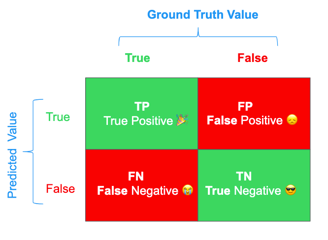
False Positive also called as Type I Error.

False Negative also called as Type II Error.

Accuracy:

It is the most straightforward and lay person-friendly metric. It will help us to understand “How accurate your model is”

Accuracy = (TP + TN)/(TP+TN+FP+FN)

Example:

If you build a binary classifier on 100 samples of balanced data, if you classify 70 classes correctly, then your accuracy is 70%. If your model classifies 95 classes correctly then accuracy is 95%.

When to use:

As mentioned above, either we have well-balanced data of positive & negative classes, or we can use the Accuracy metric after properly balancing data with imbalance data sampling techniques.

Caveats:

What if you build a basic model that always says a transaction is not fraudulent in a “Fraud Detection” model but in reality only 6% of transactions are fraudulent. What is your accuracy here? Yes, you are correct the accuracy is 94%. This is the clear drawback of accuracy; it is not suited to imbalanced and skewed data problems.

Let’s look at our next metric “Precision”.

Precision (P):

When you are trying to understand and quantify “What proportion of predicted positives are truly positives?” In another way, How many true positives are correctly identified from predicted (both TP & FP) positives?

Precision = TP /(TP + FP )

Example:

Suppose we have :

TP : 6, TN: 80, FP: 4, FN: 10

Our precision is 6/(6+4) = 0.6. i.e. Our model is correct 60 % times when it is trying to identify +ve classes. Low Precision indicates a high number of false positives.

When to Use:

If you are trying to reduce False Positives as much as possible, that means you are trying to increase Precision assuming other factors are the same. In that case, Precision is your metric. If our model has to say the sample is +ve when it is very sure and precise.

Caveats:

The model says the class is -ve (0) actually it is +ve (1)though when it is not confident. We may miss a few +ve classes because the model is not sure about those samples. It hurts when finding more +ve classes is important.

Let’s look at our next metric “Recall”.

Recall (R):

Another important metric is Recall. When you are trying to understand and quantify “What proportion of actual positives are correctly classified ?”

Recall is also called True Positive Rate (TPR) or Sensitivity.

Recall = TPR = Sensitivity = TP/ (TP + FN)

Anyhow we have talked about TPR, Let’s talk about True Negative Rate (TNR) which is known as “Specificity ”. We can talk about Specificity in the later stages of this blog.

Example:

With the same example mentioned in Precision, what is our Recall? Recall is 6/(6+10) = 0.375. This means our model identified 37.5 % of positive samples correctly.

Low Recall indicates a high number of false negatives.

When to Use:

If you are trying to reduce False Negatives as much as possible, that means you are trying to increase Recall assuming other factors are the same. In that case, Recall is your metric.

E.g. — Most standard “Cancer Prediction” problems need more Recall because FNs are more expensive here hence they become ignorant of test results even though they have cancer.

Caveats:

The recall is 1 when we say all are fraudulent transactions. That says Recall alone is not adequate. Your precision became close to 0.

Both Precision and Recall range between 0 to 1. For a great model, both Precision and Recall should be high (as close as 1). In the above example, we got a Precision is 0.6 and a recall is 0.375. How do you balance both? How do you trade Precision and Recall? Here comes our next metric i.e. F1 Score.

F1 Score (F1):

F1 Score is a combined metric of Precision and Recall. If you want to say in simple terms then it is “harmonic mean of Precision and Recall”.

F1 Score = 2PR/(P+ R)

If want to say in positives and negatives then as below:

F1 Score = 2TP/( 2TP + FP + FN)

It also ranges between 0 to 1 like Precision and Recall.

Example:

With the same example above, what is our F1 Score? Precision is 0.6 and Recall is 0.375. F1 score is (2* 0.6* 0.375)/(0.6 +0.375) = 0.46

When to use:

When dealing with datasets that have skewed targets, we should look at F1 (or precision and recall) instead of accuracy. When you need a balance between both P and R and when you need both good P and R then you need F1 Score. If your P is low then your F1 Score is low, when R is low then again F1 score is low.

Caveats:

What is 1 in F1 Score? This is actually one of the DS interview questions I personally faced in an interview. Any guesses?

The answer is 1 represents the weightage between Precision and Recall. F1 Score means Precision and Recall get equal weightage. If you pay close attention, you see that as the drawback, right? What if you want to give more weightage to Precision or Recall? There our “F Beta Score” will be our savior. Here “Beta” represents weightage between P and R. I would leave that to readers to explore. Let’s look at our next metric AUC.

AUC:

AUC represents the area under the ROC (Receiving Operating Characteristics) curve. AUC ranges between 0 to 1.

What is the ROC curve?

We already discussed the TPR and FPR in the above metrics. Let me remind you once again:

True Positive Rate (TPR) = Recall = Sensitivity = TP/(TP + FN)

False Positive Rate (FPR) = 1- TNR = 1 — Specificity = FP/(FP + TN)

If we plot TPR on the Y- axis and FPR on X- the axis with various thresholds, we will get a beautiful curve as shown below i.e. ROC curve.

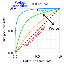
AUC = 1 represents a perfect model ideally.

AUC = 0.5 represents a random model

AUC = 0 represents very bad (very good!! If we swap target labels 0 to 1 vice versa 🙂 ) model

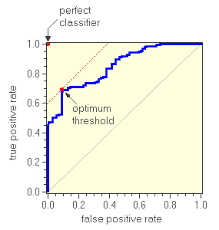
We can use the ROC curve to choose the best threshold which separates +ve and -ve classes. The ROC curve will tell you how the threshold impacts false positives and true positives. You should choose the threshold that is best suited for your business problem. Most of the time, the top-left value on the ROC curve should give you a quite good threshold. As shown in below:

Example :

When you build an Ad Click Prediction model to predict the probability of clicking an Ad. Suppose you got an AUC of 0.80. This means that if you select a random sample from your dataset which is clicked Ad (positive sample) and another random sample which is a non-clicked Ad (negative sample), then the clicking Ad sample will order/rank higher than a non-clicking Ad sample with a probability of 0.80. That order/rank is very important when displaying Ads.

Assuming it is a simple Ad prediction problem, Auction, and other ad selection standards are not required for this example purpose.

When to use:

It does not depend on thresholds like other metrics P, R, and F1. Of course, it tests all thresholds, we choose the best threshold among them.

AUC does not care about absolute probability values, it cares about the order and how well they are ranked.

If you equally care about the positive & negative classes, or the dataset is quite balanced, ROC AUC is your metric.

Caveats:

If you care more about the positive class, AUC ROC is less sensitive to the improvements for the positive class, there you may need other metrics. ex: PR AUC.

Another example is, AUC does not penalize for “how far off” the predicted score is from the actual label. For example, let’s take two positive examples (i.e., with actual label 1) that have the predicted scores of 0.55 and 0.9 at threshold 0.5. These scores will contribute equally to our loss even though one is much closer to our predicted value.

Let’s look at our next metric Log Loss.

Log Loss:

Log Loss is one of my favorite evaluation metrics. Log Loss gives importance to how well the predictions are close to the actual target. This metric captures to what degree expected probabilities diverge from class labels.

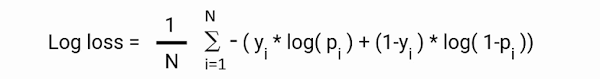
i: i th sample in the dataset.

p: prediction probability

y: ground truth of label.

N: number of samples.

The overall log loss is the pure average of an individual sample’s log loss. Log Loss is also used as an optimization function in a few ML algorithms.

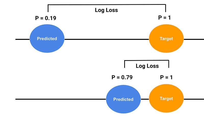
Example:

I believe this required visual representation so see below screenshot, P = 0.19 is far- off from target that is why it has high log loss. P = 0.79 is very certain about prediction so log loss is relatively minimal compared to the former one.

When to use:

log loss penalizes quite high for far-off prediction, i.e. log loss punishes you for being very sure and very wrong.

Conclusion:

Today we learned the most necessary metrics to build a classification model and trade-offs among them. Choosing the right metric always helps in finalizing the right machine-learning classification model/version for a given business problem. Otherwise, sometimes it is very hard to detect improvement in model performance even though it has really improved while training and cross-validation.

Key Takeaways:

• Tip: When your denominator is Predictive positives that is Precision. When your denominator is actual positives that is Recall.
• Precision: How many times the model is correct when it is trying to identify positive classes?
• Recall: How many positive samples are identified by our model?
• F1 Score: When you care about both P and R, want a balance between Precision and Recall.
• AUC: When you need threshold independence evaluation, and the sample’s rank/order is more important than absolute values.
• Log Loss: it considers the certainty of your predictions, it punishes you for being very sure and very wrong.

Congratulations! I believe you learned a lot today! If you have any questions, please leave a comment below.

Support this post and follow me on medium for more interesting content related to Machine Learning, MLOps, Data Science, and Experimentation!!

Disclaimer: Thanks to Google and related authors for the above illustration images.

Happy Learning!!!