
9 Tricks with Pandas that you might not know
Level up your Python competencies with Pandas

If you haven’t been living under a rock for the past decade or so, you’ve probably heard about Pandas. It’s basically Excel but 100x more powerful. Or the Pythonic equivalent to SQL.
What’s cool about Pandas is that it lets you explore and manipulate data without having to write much boilerplate code and without making your computer run hot. If you’re doing data science with Python — which, judging from the fact that you’re reading this post, you are — then Pandas is the package that your workflow starts with.
I won’t bother you with the elementary stuff; there are plenty of excellent tutorials which cover that if you need a refresher.
Here’s a few tricks that you might not have heard of yet. Okay, maybe you’ll have heard of one or two before reading this post, but hopefully you’ll learn some new nifty tricks anyway which might make your life a little easier.
For the purpose of demonstration, we’ll be using a dataset listing the causes of death in France from 2001 to 2008. This is a little bit weird and niche, I know. But it’s a good dataset for us to train on.
This is what it looks like:
>>> import pandas as pd
>>> df = pd.read_csv("CausesOfDeath_France_2001-2008.csv")
>>> df = df[["TIME", "SEX", "Value", "ICD10"]]
>>> df
      TIME    SEX    Value      ICD10
0     2001    Males  277 858    All causes of death (A00-Y89)
1     2001    Males    5 347    Certain infectious diseases
2     2001    Males      545    Tuberculosis
3     2001    Males       30    Meningococcal infection
4     2001    Males      471    Viral hepatitis
...    ...      ...      ...    ...
1051  2008  Females    2 815    Falls
1052  2008  Females      630    Accidental poisoning
1053  2008  Females    2 768    Intentional self-harm
1054  2008  Females      166    Assault
1055  2008  Females       68    Event of undetermined intent
Above I’ve filtered this data to include only columns that are of interest. The sex marker doesn’t include non-binary and intersex people, but hey, the data is old.
1. Categorical data saves time and space
We have a big fat column called ICD10 which contains lots of strings. These take up quite a lot of storage space…
>>> df.info()
<class 'pandas.core.frame.DataFrame'>
RangeIndex: 1056 entries, 0 to 1055
Data columns (total 4 columns):
#   Column  Non-Null Count  Dtype
---  ------  --------------  -----
0   TIME    1056 non-null   int64
1   SEX     1056 non-null   object
2   Value   1056 non-null   object
3 ICD10 1056 non-null objectdtypes: int64(1), object(3)
memory usage: 33.1+ KB>>> df.memory_usage(deep=True)
Index 128
TIME 8448
SEX 66528
Value 64758
ICD10 101840
dtype: int64This particular dataset only has 1056 columns, so the entire memory consumption isn’t terrible. However, when you have millions of columns, you wouldn’t want to have to contend with gigabytes of RAM.
We can make this better by using factorize():
>>> number, icd10 = pd.factorize(df["ICD10"])
>>> number
array([ 0,  1,  2, ..., 63, 64, 65])
>>> icd10
Index(['All causes of death (A00-Y89) excluding S00-T98',
'Certain infectious and parasitic diseases (A00-B99)', 'Tuberculosis',
'Meningococcal infection',
'Viral hepatitis',
...,
'Falls',
'Accidental poisoning by and exposure to noxious substances',
'Intentional self-harm',
'Assault',
'Event of undetermined intent'],
dtype='object')
What we did here is we encoded the contents of ICD10 in an array of numbers. Instead of using the original column of strings we can now use the newly-created column number and save space:
>>> df['ICD10'] = number
>>> df
      TIME      SEX    Value  ICD10
0     2001    Males  277 858      0
1     2001    Males    5 347      1
2     2001    Males      545      2
3     2001    Males       30      3
4     2001    Males      471      4
...    ...      ...      ...    ...
1051  2008  Females    2 815     61
1052  2008  Females      630     62
1053  2008  Females    2 768     63
1054  2008  Females      166     64
1055 2008 Females 68 65[1056 rows x 4 columns]Our memory usage for ICD10 goes markedly down:
>>> df.memory_usage(deep=True)
Index      128
TIME      8448
SEX      66528
Value    64758
ICD10     8448
dtype: int64
This might not seem like a big deal with such a small dataset; with larger ones, however, this can save tons of resources.
One caveat with this method is that if you want to add a new category in the factorized column, you’ll have to update the objects you’ve factorized (in our case number and icd10). This helps when you re-convert the factorized column back into strings by using number and icd10 like a map.
2. Making histograms and other plots
It’s quite easy to make histograms with Pandas. All we need is a little help from Matplotlib:
import matplotlib.pyplot as plt
hist = df['ICD10'].hist(bins=66); plt.show()
This histogram isn’t worth showing; it’s essentially a straight line at y=16. This makes sense because all 66 causes of mortality are listed over 8 years for 2 sexes. Hence we have 16 entries per cause of mortality.
We might want to make a more interesting plot though. How about plotting evolution of the all-cause mortality over time?
We have encoded the all-cause mortality as 0 in our first step. So we’ll filter those data points:
df1 = df[(df['ICD10'] == 0) & (df['SEX'] == 'Females')]
df2 = df[(df['ICD10'] == 0) & (df['SEX'] == 'Males')]
We can now show the all-cause mortality over time:
>>> plt.plot(df1['TIME'], df1['Value'], label='Females')
>>> plt.plot(df2['TIME'], df2['Value'], label='Males')
>>> plt.legend()
>>> plt.title('All-cause mortality in France')
>>> plt.show()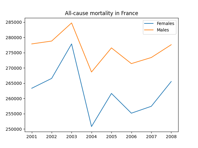
Conclusion from this plot: Ladies don’t die as much as gentlemen do! The peak from 2003, by the way, is due to a massive heatwave which hit France unprepared and caused heatstrokes and other fatalities of many elderly people that year.
With a little bit of help from Matplotlib, making plots of Pandas objects is a charm. Imagine how much more lines of code you would have needed using some arrays instead of Pandas!
3. Bin your data with membership mapping
Remember the column ICD10 which we replaced by a code of numbers earlier on?
Sometimes we don’t want to convert it back to the original strings, but rather group some data together. Maybe we’re particularly interested in causes of death from infectious diseases, or the consequences of bad mental health. Some preliminary grouping might look like this:
>>> groups = {'Infectious diseases': ('1', '2', '3', '4', '5', '32', '38'), 'Neoplasms': ('6', '7', '8', '9', '10', '11', '12', '13', '14', '15', '16', '17', '18', '19', '20', '21', '22', '23', '24'), 'Endocrine': ('26', '27'), 'Mental & Drugs': ('28', '29', '30', '62', '63'), 'Lungs': ('39', '40', '41'), 'Stomach, Liver, Kidney': ('42', '43', '44', '48'), 'Childbirth': ('50', '51'), 'Congenital stuff': ('52', '53', '54', '56'), 'External': ('58', '59', '60', '61', '62', '64')}Don’t check this up too closely against the list of causes of death from the dataset; I’m not a medical professional. My judgement is, quite likely, flawed.
Now we can match this against our column ICD10 by using this nifty function which I stole from some genius at Realpython:
>>> from typing import Any>>> def membership_map(s: pd.Series, groups: dict,
... fillvalue: Any=-1) -> pd.Series:
... # Reverse & expand the dictionary key-value pairs
... groups = {x: k for k, v in groups.items() for x in v}
... return s.map(groups).fillna(fillvalue)>>> df['ICD10'] = df['ICD10'].astype('string')>>> membership_map(df['ICD10'], groups, fillvalue='other')
0 other
1 Infectious diseases
2 Infectious diseases
3 Infectious diseases
4 Infectious diseases
...
1051 External
1052 External
1053 Mental & Drugs
1054 External
1055 other
Name: ICD10, Length: 1056, dtype: objectNote the fact that we converted the data type of ICD10 to a string to make this match the string literals from the dictionary groups. Just using integers in the definition of groups won’t work because Python can’t iterate over those.
4. Load data from the clipboard
Did you know that you can literally create a Pandas DataFrame from the clipboard? This is handy for example when a colleague has given you an Excel spreadsheet with data which you’d like to process in Pandas.
As an example, I’ll use the first 10 rows of our example dataset:
>>> df[:10]
   TIME    SEX   Value ICD10
0  2001  Males  277858     0
1  2001  Males    5347     1
2  2001  Males     545     2
3  2001  Males      30     3
4  2001  Males     471     4
5  2001  Males     892     5
6  2001  Males   91737     6
7  2001  Males   88481     7
8  2001  Males    3755     8
9  2001  Males    3442     9
Now, all I need to do is copy this data to my clipboard. I create a new DataFrame from my clipboard like this:
df10 = pd.read_clipboard()Nifty, huh?
5. Get quick stats
What if we wanted to know a few key features of our data set? We have used df.info() and df.memory_usage() above, but these methods are quite technical and don’t tell us much about the data itself.
If we want to get more data science insights, don’t look further than df.describe:
>>> df.describe(include='all')
               TIME    SEX          Value        ICD10
count   1056.000000   1056    1056.000000  1056.000000
unique          NaN      2            NaN          NaN
top             NaN  Males            NaN          NaN
freq            NaN    528            NaN          NaN
mean    2004.500000    NaN   12069.661932    32.500000
std        2.292374    NaN   35896.576873    19.059398
min     2001.000000    NaN       0.000000     0.000000
25%     2002.750000    NaN     479.500000    16.000000
50%     2004.500000    NaN    2606.000000    32.500000
75%     2006.250000    NaN    7729.500000    49.000000
max     2008.000000    NaN  284729.000000    65.000000
With the option include='all' you ensure that non-numerical data types don’t get ignored. Note that non-numerical data types don’t have entries for mean through max — because what’s the mean or the maximum value of a bunch of words? Similarly, the fields unique, top, and freq are not applicable for numerical types.
Getting basic insights doesn’t get easier than this.
6. Query instead of conditional statements
We might want to find out which causes of death are quite rare in France. We’ll define rare as happening at least once and at most 50 times per year for each gender. (This is not official medical jargon of course; it just fits well for this data set.)
Instead of messing around with a conditional mask like df[0 < df['Value'] < 50], you use query() and make your commands shorter:
>>> df.query('0 < Value < 50')This is still a fairly long list but we can condense it by listing only the causes of death which appeared on it:
>>> df.query('0 < Value < 50').ICD10.unique()
array([ 3, 30, 50])
The result corresponds to meningococcal infection, drug dependence, and pregnancy. In the measured time period, no men died from pregnancy-related issues, though. Yes, I am aware that it’s statistically unlikely, though not impossible, for men to get pregnant 🙂
7. Group your data
One of the most powerful functions in Pandas is by far groupby(). We’ll use this to find out which causes of death happened the most often.
For this I create another data frame which does not contain the numbers for the all-cause mortality (which would obviously be the highest number). Then I group the entries by value to see what results in the highest and lowest mortality:
>>> dfno0 = df.query('ICD10!=0')
>>> dfno0.groupby('Value').first()
       TIME      SEX  ICD10
Value
0      2001    Males     18
12     2005    Males      3
14     2006    Males      3
15     2001  Females      3
17     2006  Females      3
...     ...      ...    ...
92631  2003    Males      6
93207  2006    Males      6
93550  2005    Males      6
93773  2007    Males      6
93872 2008 Males 6[930 rows x 3 columns]We get that cause 6 is the most deadly, which is neoplasms. In other words, tumors, cancer and stuff like that.
If we want a more detailed overview and don’t want to scroll through too much data, however, something without groupby() is needed.
>>> dfno0.sort_values(by=['Value'], ascending=False).drop_duplicates('ICD10').head(5)
     TIME      SEX  Value  ICD10
930  2008    Males  93872      6
931  2008    Males  90481      7
363  2003  Females  87738     33
365  2003  Females  27084     35
322  2003    Males  25133     58
This sorts the death numbers from highest to lowest, and drops rows where the ICD10 code appears more than once. We therefore see the top 5 causes of death in the timeframe we considered. They correspond to neoplasms (cancer-related stuff), malignant neoplasms (cancer-related stuff again), diseases of the circulatory system, other heart diseases, and external causes of death.
This last overview, however, was much more elaborate. With groupby you’re able to get a quick and dirty overview in record time.
8. Make your data explode 🙂
For the purpose of this section, we’ll use a dummy dataset. Have you seen data sets like this before?
>>> df2 = pd.DataFrame({'A': [1, 2, 3], 'B':[1, 2, [3, 4, 5]]})The author of this dataset presumably didn’t want it to look this messy:
>>> df2
   A          B
0  1          1
1  2          2
2  3  [3, 4, 5]
Luckily, we can explode() this last ugly entry:
>>> df2.explode('B')
   A  B
0  1  1
1  2  2
2  3  3
2  3  4
2  3  5
Congratulations, you have encountered the first time in the world where an explosion made the world tidier, not messier 🙂
9. Write Pandas objects directly to compressed files
When you’ve painstakingly messed about with your data, you might want to save your Pandas objects before you grab a beer and call it a day. Most people save their Series and DataFrames as CSV files. They might compress those to save disk space.
Well, if you want to be a little bit extra, you can compress your CSV files.
This is how it works:
>>> df.to_csv('df.csv.gz', compression='gzip')You’re welcome 🙂
Famous last words
Pandas is a fantastic tool for straightforward data cleaning and management. Of course you can do all this in SQL and in whichever programming language you prefer, but there are reasons why Pandas is so popular among data scientists.
The hidden gems I showed in this article are just a few of them.
Become a Medium member for full access to my content.
Level Up Coding
Thanks for being a part of our community! Before you go:
- 👏 Clap for the story and follow the author 👉
- 📰 View more content in the Level Up Coding publication
- 🔔 Follow us: Twitter | LinkedIn | Newsletter
🚀👉 Join the Level Up talent collective and find an amazing job