
70%+ Automated Returns-15M Bull Reversal-NQ Futures
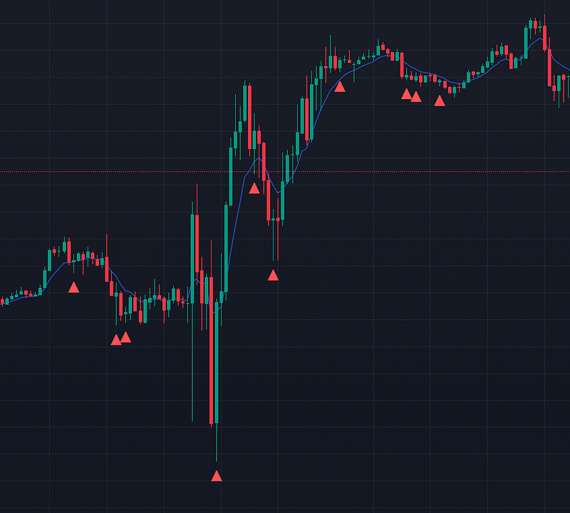
This article will present the code to execute a simple 15m candle reversal patten on Nasdaq futures using Python. The pattern essentially detects selling exhaustion in the market, leaving a higher probability of price moving in the other direction. The criteria for the reversal pattern is as follows: a bearish candle must precede a bullish candle with a lower low, a lower high and a close within the body of the bear candle. Then, the code runs a simulation that enters a trade one tick above the high of the signal candle with a 35-tick profit/loss; i.e. a 1:1 Risk Reward Ratio with no time limit. This means whenever the signal is generated, the trade order will remain open until price reaches this level.
// Pine Script for implementing in TradingView
//@version=4
study("Candlestick Patterns", shorttitle="CP", overlay=true)

// Identify Bear Candle
bearCandle = close[1] < open[1]

// Check for Bull Candle with specific criteria
bullCandleCriteria = close > open and close > close[1] and close < open[1] and low < low[1] and high < high[1]

// Combine conditions to detect the specified pattern for bear followed by bull
bearBullPattern = bearCandle and bullCandleCriteria

// Plot yellow triangle on the second candle of the bear followed by bull pattern as a signal indicator
plotshape(bearBullPattern, style=shape.triangleup, location=location.belowbar, color=color.red, size=size.small)
I have also generated plots to show which time of day this strategy works best and worst, as well as the daily win/loss percentage. Lastly, I wanted to test if there was a significant success rate for this setup with respect to an 8-period Exponential Moving Average.
I coded all of this into Google Colab using Python and collected data from TradingView. The dataset is over 20000 periods long, spanning 10 months 2023–05–01 00:00:00 to 2024–03–13 20:15:00.
!pip install yfinance pandas matplotlib mplfinance

# Mounting T Data Sets from Google Drive

from google.colab import drive
drive.mount('/content/drive')

# Path to your file, e.g., "My Drive" is the root directory of your Google Drive
file_path = '/content/drive/My Drive/Historical_T_Data/NQ_15M_ETH.csv'

import pandas as pd
df = pd.read_csv(file_path, header = None)

# Define the conditions for the original signal pattern
def detect_signal_pattern(df):
    # Identify Bear Candle
    df['bearCandle'] = df[4] < df[1]

    # Check for Bull Candle with specific criteria
    bull_candle_condition = (
        (df[3] < df[3].shift(1)) &
        (df[2] < df[2].shift(1)) &
        (df[4] < df[1].shift(1)) &
        (df[4] > df[4].shift(1))
    )
    df['bullCandle'] = bull_candle_condition

    # Combine conditions to detect the original signal pattern
    df['signalPattern'] = df['bearCandle'].shift(1) & df['bullCandle']

    return df

# Define the conditions for the opposite signal pattern
def detect_opposite_signal_pattern(df):
    # Identify Bull Candle
    df['bullCandleOpposite'] = df[4] > df[1]

    # Check for Bear Candle with specific criteria
    bear_candle_condition = (
        (df[3] > df[3].shift(1)) &
        (df[2] > df[2].shift(1)) &
        (df[4] > df[1].shift(1)) &
        (df[4] < df[4].shift(1))
    )
    df['bearCandleOpposite'] = bear_candle_condition

    # Combine conditions to detect the opposite signal pattern
    df['oppositeSignalPattern'] = df['bullCandleOpposite'].shift(1) & df['bearCandleOpposite']

    return df

# Load your dataset into a DataFrame (replace this with your actual dataset)
# Assuming your dataset is already loaded into df

# Apply the indicator functions to your dataset
df = detect_signal_pattern(df)
df = detect_opposite_signal_pattern(df)

# Print the modified DataFrame with signal pattern columns
print(df)
import pandas as pd

# Function to apply the strategy and calculate performance metrics
def apply_strategy(df):
    # Initialize variables for performance metrics
    total_trades = 0
    total_winning_trades = 0
    total_losing_trades = 0

    # Iterate over rows in the DataFrame
    for index, row in df.iterrows():
        # Check if there is a bull signal
        if row['bullCandle']:
            # Convert values to numeric
            high = pd.to_numeric(row[2])

            # Take long position one tick above the high of the bull signal candle
            entry_price = high + 0.01

            # Increment total trades count
            total_trades += 1

            # Initialize variables to track price movement
            max_high = entry_price
            min_low = entry_price

            # Iterate over subsequent rows to track price movement
            for next_index, next_row in df.iloc[index+1:].iterrows():
                # Convert values to numeric
                next_high = pd.to_numeric(next_row[2])
                next_low = pd.to_numeric(next_row[3])

                # Update max_high and min_low
                max_high = max(max_high, next_high)
                min_low = min(min_low, next_low)

                # Check if price rises by 35 ticks first
                if max_high - entry_price >= 35 * 0.01:
                    total_winning_trades += 1
                    break
                # Check if price drops by 35 ticks first
                elif entry_price - min_low >= 35 * 0.01:
                    total_losing_trades += 1
                    break

    # Calculate win rate percentage
    win_rate_percentage = (total_winning_trades / total_trades) * 100 if total_trades != 0 else 0

    # Print performance metrics
    print("Total Trades Taken:", total_trades)
    print("Number of Winners:", total_winning_trades)
    print("Number of Losers:", total_losing_trades)
    print("Win Rate Percentage:", win_rate_percentage)

# Load your dataset into a DataFrame (replace this with your actual dataset)
# Assuming your dataset is already loaded into df

# Apply the strategy and calculate performance metrics
apply_strategy(df)
Total Trades Taken: 1080 Number of Winners: 758 Number of Losers: 322 Win Rate Percentage: 70.185%
import pandas as pd

# Function to apply the strategy and return winning and losing trades
def get_trades(df):
    winning_trades = []
    losing_trades = []

    # Iterate over rows in the DataFrame
    for index, row in df.iterrows():
        # Check if there is a bull signal
        if row['bullCandle']:
            # Convert values to numeric
            high = pd.to_numeric(row[2])

            # Take long position one tick above the high of the bull signal candle
            entry_price = high + 0.01

            # Initialize variables to track price movement
            max_high = entry_price
            min_low = entry_price

            # Iterate over subsequent rows to track price movement
            for next_index, next_row in df.iloc[index+1:].iterrows():
                # Convert values to numeric
                next_high = pd.to_numeric(next_row[2])
                next_low = pd.to_numeric(next_row[3])

                # Update max_high and min_low
                max_high = max(max_high, next_high)
                min_low = min(min_low, next_low)

                # Check if price rises by 35 ticks first
                if max_high - entry_price >= 35 * 0.01:
                    winning_trade_data = {'EntryPrice': entry_price, 'ExitPrice': max_high}
                    winning_trade_data.update(row)  # Add original row data
                    winning_trades.append(winning_trade_data)
                    break
                # Check if price drops by 35 ticks first
                elif entry_price - min_low >= 35 * 0.01:
                    losing_trade_data = {'EntryPrice': entry_price, 'ExitPrice': min_low}
                    losing_trade_data.update(row)  # Add original row data
                    losing_trades.append(losing_trade_data)
                    break

    # Create DataFrames for winning and losing trades
    winning_trades_df = pd.DataFrame(winning_trades)
    losing_trades_df = pd.DataFrame(losing_trades)

    return winning_trades_df, losing_trades_df

# Load your dataset into a DataFrame (replace this with your actual dataset)
# Assuming your dataset is already loaded into df

# Get winning and losing trades
winning_trades_df, losing_trades_df = get_trades(df)

# Print winning trades DataFrame
print("Winning Trades:")
print(winning_trades_df)

# Print losing trades DataFrame
print("\nLosing Trades:")
print(losing_trades_df)


import pandas as pd

# Function to tally winning trades in each hour
def tally_winning_trades_by_hour(winning_trades_df):
    # Convert the 'date' column to datetime with timezone awareness
    winning_trades_df['date'] = pd.to_datetime(winning_trades_df[0], utc=True)

    # Convert to local timezone (adjust as per your data)
    winning_trades_df['date'] = winning_trades_df['date'].dt.tz_convert('Europe/London')

    # Extract hour from the timestamp
    winning_trades_df['hour'] = winning_trades_df['date'].dt.hour

    # Group the trades by hour and count the number of winning trades in each hour
    hourly_counts = winning_trades_df.groupby('hour').size()

    return hourly_counts

# Assuming winning trades DataFrame is already loaded and named winning_trades_df

# Tally winning trades in each hour
hourly_counts = tally_winning_trades_by_hour(winning_trades_df)

# Print the hourly counts
print("Winning Trades Tally by Hour:")
print(hourly_counts)

#########

import pandas as pd
import matplotlib.pyplot as plt

# Function to tally winning trades in each hour
def tally_winning_trades_by_hour(winning_trades_df):
    # Convert the 'date' column to datetime with timezone awareness
    winning_trades_df['date'] = pd.to_datetime(winning_trades_df['date'], utc=True)

    # Convert to local timezone (adjust as per your data)
    winning_trades_df['date'] = winning_trades_df['date'].dt.tz_convert('Europe/London')

    # Extract hour from the timestamp
    winning_trades_df['hour'] = winning_trades_df['date'].dt.hour

    # Group the trades by hour and count the number of winning trades in each hour
    hourly_counts = winning_trades_df.groupby('hour').size()

    return hourly_counts

# Assuming winning trades DataFrame is already loaded and named winning_trades_df

# Tally winning trades in each hour
hourly_counts = tally_winning_trades_by_hour(winning_trades_df)

# Plot a bar chart
hourly_counts.plot(kind='bar', figsize=(10, 6))
plt.title('Tally of Winning Trades by Hour')
plt.xlabel('Hour')
plt.ylabel('Number of Winning Trades')
plt.xticks(rotation=45)
plt.grid(axis='y', linestyle='--', alpha=0.7)
plt.show()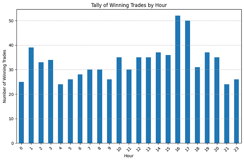
import pandas as pd

# Function to tally losing trades in each hour
def tally_losing_trades_by_hour(losing_trades_df):
    # Convert the 'date' column to datetime with timezone awareness
    losing_trades_df['date'] = pd.to_datetime(losing_trades_df[0], utc=True)

    # Convert to local timezone (adjust as per your data)
    losing_trades_df['date'] = losing_trades_df['date'].dt.tz_convert('Europe/London')

    # Extract hour from the timestamp
    losing_trades_df['hour'] = losing_trades_df['date'].dt.hour

    # Group the trades by hour and count the number of losing trades in each hour
    hourly_counts = losing_trades_df.groupby('hour').size()

    return hourly_counts

# Assuming losing trades DataFrame is already loaded and named losing_trades_df

# Tally losing trades in each hour
hourly_counts_losing = tally_losing_trades_by_hour(losing_trades_df)

# Print the hourly counts
print("Losing Trades Tally by Hour:")
print(hourly_counts_losing)

import matplotlib.pyplot as plt

# Plot a bar chart for losing trades by hour
hourly_counts_losing.plot(kind='bar', figsize=(10, 6), color='red')
plt.title('Tally of Losing Trades by Hour')
plt.xlabel('Hour')
plt.ylabel('Number of Losing Trades')
plt.xticks(rotation=45)
plt.grid(axis='y', linestyle='--', alpha=0.7)
plt.show()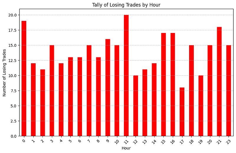
import pandas as pd

# Function to tally winning trades by day of the week
def tally_winning_trades_by_day(winning_trades_df):
    # Convert the 'date' column to datetime with timezone awareness
    winning_trades_df['date'] = pd.to_datetime(winning_trades_df['date'], utc=True)

    # Convert to local timezone (adjust as per your data)
    winning_trades_df['date'] = winning_trades_df['date'].dt.tz_convert('Europe/London')

    # Extract day of the week from the timestamp
    winning_trades_df['day_of_week'] = winning_trades_df['date'].dt.day_name()

    # Group the trades by day of the week and count the number of winning trades for each day
    daily_counts = winning_trades_df.groupby('day_of_week').size()

    return daily_counts

# Function to tally losing trades by day of the week
def tally_losing_trades_by_day(losing_trades_df):
    # Convert the 'date' column to datetime with timezone awareness
    losing_trades_df['date'] = pd.to_datetime(losing_trades_df['date'], utc=True)

    # Convert to local timezone (adjust as per your data)
    losing_trades_df['date'] = losing_trades_df['date'].dt.tz_convert('Europe/London')

    # Extract day of the week from the timestamp
    losing_trades_df['day_of_week'] = losing_trades_df['date'].dt.day_name()

    # Group the trades by day of the week and count the number of losing trades for each day
    daily_counts = losing_trades_df.groupby('day_of_week').size()

    return daily_counts

# Assuming winning trades and losing trades DataFrames are already loaded and named winning_trades_df and losing_trades_df respectively

# Tally winning trades by day of the week
daily_counts_winning = tally_winning_trades_by_day(winning_trades_df)

# Tally losing trades by day of the week
daily_counts_losing = tally_losing_trades_by_day(losing_trades_df)

# Print the daily counts for winning trades
print("Winning Trades Tally by Day of the Week:")
print(daily_counts_winning)
print()

# Print the daily counts for losing trades
print("Losing Trades Tally by Day of the Week:")
print(daily_counts_losing)

import matplotlib.pyplot as plt

# Plot a bar chart for winning trades by day of the week
plt.figure(figsize=(10, 6))
daily_counts_winning.plot(kind='bar', color='green', alpha=0.7, label='Winning Trades')

# Plot a bar chart for losing trades by day of the week
daily_counts_losing.plot(kind='bar', color='red', alpha=0.7, label='Losing Trades')

# Customize the plot
plt.title('Tally of Trades by Day of the Week')
plt.xlabel('Day of the Week')
plt.ylabel('Number of Trades')
plt.legend()
plt.xticks(rotation=45)
plt.grid(axis='y', linestyle='--', alpha=0.7)
plt.tight_layout()

# Show the plot
plt.show()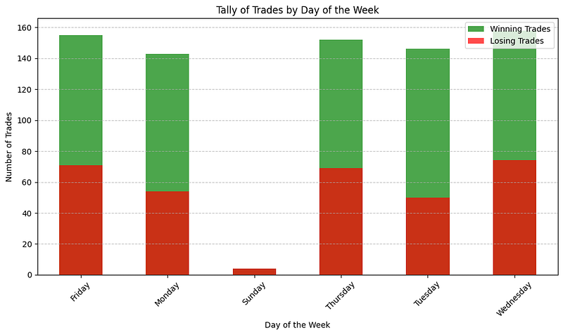
# Convert the 'EMA' column to numerical values
df['EMA'] = pd.to_numeric(df[6], errors='coerce')

# Check if the buy price is above or below the EMA for each trade
df['buy_price_above_EMA'] = df['entry_price'] > df['EMA']

# Now calculate the percentage of winners where the price is above and below the EMA
winners_above_EMA = df[df['signalPattern'] & df['buy_price_above_EMA']]
winners_below_EMA = df[df['signalPattern'] & ~df['buy_price_above_EMA']]

percentage_winners_above_EMA = (len(winners_above_EMA) / len(df[df['signalPattern']])) * 100
percentage_winners_below_EMA = (len(winners_below_EMA) / len(df[df['signalPattern']])) * 100

# Print the percentages
print("Percentage of winners where the price is above EMA:", percentage_winners_above_EMA)
print("Percentage of winners where the price is below EMA:", percentage_winners_below_EMA)
Percentage of winners where the price is above EMA: 51.67 Percentage of winners where the price is below EMA: 48.33


