7 Pandas Hacks That Every AI Expert Should Know

Unlock AI & Data Science Mastery with Top Pandas Hacks

Created with Abidin Dino AI, to reach it, consider being Paid subscriber to LearnAIWithMe, here

“In the age of artificial intelligence, being smart will mean something completely different.”

Ginni Rometty

Ginni is highlighting the shift towards a new paradigm of intelligence augmented by technology.

Bridging this evolution, Pandas stands as an essential library for AI experts, empowering them with functions that streamline data analysis and enhance machine learning workflows.

Through mastering advanced Pandas hacks in this article, you will unlock deeper insights and efficiencies, propelling your AI projects to new heights.

Effortless Merging of Datasets

Merging datasets is a fundamental task in data science, often necessary for combining information from multiple sources. While the traditional merge operation is powerful, it can sometimes feel verbose.

Normal Version

Traditional Merge Operations with pd.merge()

The pd.merge() function is a versatile tool for combining datasets based on common columns or indices. Here’s a conventional way of using it:

import pandas as pd

# Sample datasets: Books and their respective sales
books = pd.DataFrame({
    'BookID': [1, 2, 3],
    'Title': ['Python Fundamentals', 'Advanced Machine Learning', 'Data Science for Beginners']
})

sales = pd.DataFrame({
    'BookID': [1, 2, 3],
    'UnitsSold': [500, 300, 800]
})

# Merging datasets using pd.merge()
merged_df = pd.merge(books, sales, on='BookID')

print(merged_df)

Here is the output.

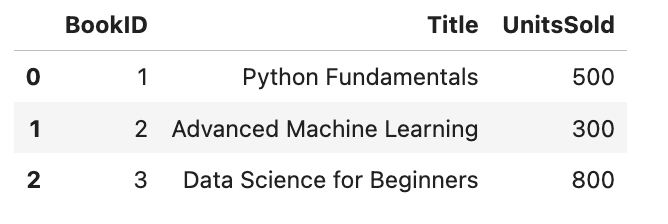
This method works well but involves specifying the DataFrame to merge, the type of join, and the keys on which to join, which can be a bit lengthy for some.

Hacked Version

Streamlining Data Merges with DataFrame.join() for Improved Syntax and Performance

For a simpler syntax and often better performance, especially for index-based joins, you can use the DataFrame.join() method. It provides a more concise way to merge DataFrames, particularly when the DataFrames are already aligned on the index.

# Setting the index to 'BookID' for both DataFrames
books_indexed = books.set_index('BookID')
sales_indexed = sales.set_index('BookID')

# Merging datasets using join()
simplified_merged_df = books_indexed.join(sales_indexed)

simplified_merged_df

Here is the output.

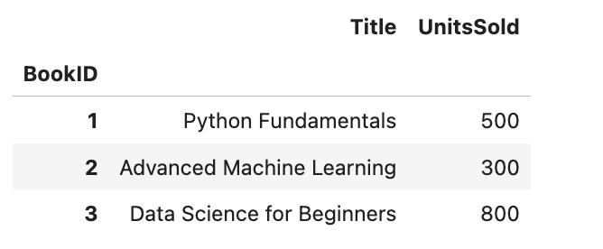
By aligning our DataFrames on a common index and using .join(), we simplify the merge operation, which is not only enhances readability but also leverages the efficiency of index-based operations in Pandas.

Dynamic Data Aggregation Made Simple

Aggregating data is akin to distilling raw information into potent insights. While the standard approach gets the job done, there’s a dynamic twist that can elevate your data analysis game.

Normal Version

Basic Usage of groupby() Followed by Aggregate Functions

Pandas’ groupby() is the bread and butter for data aggregation, allowing us to group data and apply functions like sum, mean, etc. Here’s the usual way it’s done:

import pandas as pd

# Sample sales data by product category
data = {
    'Category': ['Books', 'Electronics', 'Books', 'Electronics'],
    'Sales': [150, 200, 550, 1200]
}
df = pd.DataFrame(data)

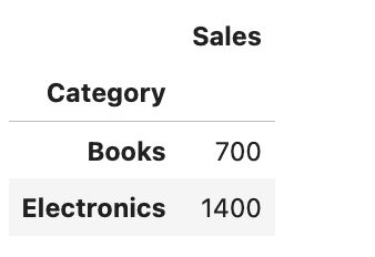
# Aggregating sales by category using groupby()
grouped_df = df.groupby('Category').sum()

grouped_df

Here is the output.

Hacked Version

Applying agg() with Custom Lambda Functions for Powerful Inline Aggregations

Now, let’s kick things up a notch with the agg() function, which allows for more complex and tailored aggregations using lambda functions. This method shines when you need to perform multiple, distinct aggregations simultaneously:

# Aggregating with custom functions using agg()
custom_agg_df = df.groupby('Category').agg({
    'Sales': [('TotalSales', 'sum'), ('AverageSales', 'mean'), ('MaxSale', 'max')]
})

custom_agg_df

Here is the output.

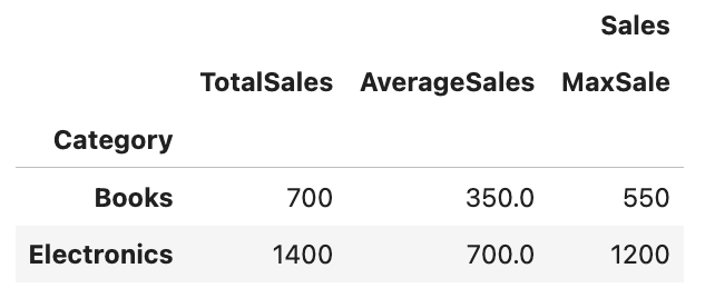
By using agg() with a dictionary specifying the operations for each column, we can easily perform complex aggregations in a single step.

This not only makes our code more concise but also unlocks a higher level of data analysis flexibility.

Note : Custom lambda functions can further tailor these operations, providing precise control over the aggregation logic.

Rapid Value Counts for Data Exploration

Understanding the distribution of values within your data is crucial for initial analysis and insight generation. While the basic use of value_counts() is widely known, there’s a hack that can provide even more depth to this exploration.

Normal Version

Utilizing value_counts() for Single Column Analysis

The value_counts() method is a quick and easy way to see the distribution of values in a column. Here's the standard way to use it:

import pandas as pd

# Sample data: Product categories
data = {'Category': ['Books', 'Electronics', 'Books', 'Books', 'Electronics', 'Gadgets']}
df = pd.DataFrame(data)

# Using value_counts to analyze category distribution
category_counts = df['Category'].value_counts()

print(category_counts)

Here is the output.

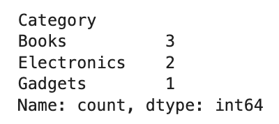
This method gives us a straightforward count of each category, which is very useful for quick insights into categorical data distribution.

Hacked Version

Extending value_counts() with normalize=True for Proportion Analysis

To understand not just the count but also the proportion of each category within the dataset, you can use the normalize parameter of value_counts(). This provides a clearer picture of the data's composition:

# Analyzing category distribution with proportions
category_proportions = df['Category'].value_counts(normalize=True)

category_proportions

Here is the output.

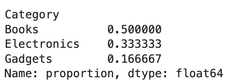
This insight is particularly valuable when comparing distributions across datasets of different sizes or when you need to communicate the relative importance of categories.

Cleaning Data with Efficient Missing Values Handling

Dealing with missing values is an inevitable part of data preprocessing. While there are several ways to identify missing data, optimizing this process can save both time and ensure cleaner datasets.

Normal Version

Using isnull() to Find Missing Values

The isnull() method in Pandas is a standard approach for detecting missing values in a DataFrame. It returns a boolean DataFrame indicating whether each value is missing. Here's how it's typically applied:

import pandas as pd
import numpy as np

# Sample data with missing values
data = {
    'Name': ['Alice', 'Bob', 'Charlie', 'David', 'Eve'],
    'Age': [25, np.nan, 30, np.nan, 22],
    'Salary': [50000, 60000, np.nan, 55000, np.nan]
}
df = pd.DataFrame(data)

# Finding missing values
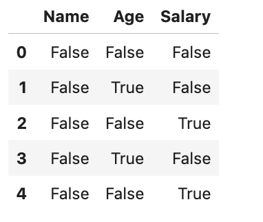
missing_values = df.isnull()

missing_values

Here is the output.

Hacked Version

Combining isnull() with fillna() for In-place Data Cleaning

A more streamlined approach involves not just finding but also replacing missing values in one go. This is where fillna() comes into play, allowing you to fill missing values with a specified number, method, or even a forward-fill or back-fill to carry the next or previous values forward.

# Filling missing values with a specified value
df_filled = df.fillna({
    'Age': df['Age'].mean(),  # Replace missing ages with the average age
    'Salary': 0  # Assume missing salary as 0 for simplification
})

df_filled

Here is the output.

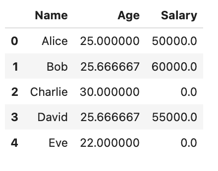
By combining isnull() with fillna(), we not only identify but also rectify missing values in our dataset, ensuring a more streamlined data-cleaning process.

This method enhances the dataset's integrity, making it ready for analysis or machine learning algorithms without additional steps for handling missing data.

Duplicate Detection and Removal for Data Integrity

Ensuring the uniqueness of data is essential for accurate analysis. While detecting duplicates is straightforward with Pandas, there’s a refined method that not only identifies but also selectively removes duplicates, preserving data integrity.

Normal Version

Identifying Duplicates with duplicated()

The duplicated() function in Pandas marks duplicate rows, allowing for their identification. It’s a first step in cleaning data duplicates. Here's how it is typically used:

import pandas as pd

# Sample data with potential duplicates
data = {
    'Name': ['Alice', 'Bob', 'Charlie', 'Alice', 'Bob'],
    'Age': [25, 30, 35, 25, 30],
    'City': ['New York', 'Los Angeles', 'Chicago', 'New York', 'Los Angeles']
}
df = pd.DataFrame(data)

# Identifying duplicates
duplicates = df.duplicated()

duplicates

Here is the output.

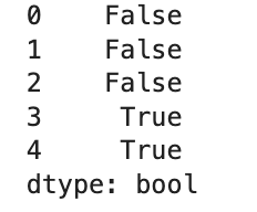
While duplicated() is useful for spotting duplicates, it doesn’t remove them. Let’s explore how to take this a step further.

Hacked Version

Employing drop_duplicates() with Subset Argument to Target Specific Columns

To not only identify but also remove duplicates, we use drop_duplicates(). This function can be fine-tuned with the subset argument to specify columns for finding duplicates, offering a powerful way to clean your dataset.

# Removing duplicates with specificity
cleaned_df = df.drop_duplicates(subset=['Name', 'City'])

cleaned_df

Here is the output.

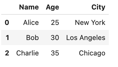
This approach not only cleans the data but does so with precision, ensuring the integrity and utility of our dataset for analysis.

Seamless Data Visualization Directly from Pandas

Data visualization is a powerful tool for understanding complex datasets at a glance. While Pandas offers basic plotting capabilities, there’s a hack that can make creating diverse types of visualizations even more seamless.

Normal Version

Basic Plotting with Pandas

Pandas integrates with Matplotlib to offer a straightforward way to plot your data directly from DataFrame objects. Here’s a simple example:

import pandas as pd
import matplotlib.pyplot as plt

# Sample data: Sales over a week
data = {
    'Day': ['Monday', 'Tuesday', 'Wednesday', 'Thursday', 'Friday'],
    'Sales': [200, 300, 400, 350, 500]
}
df = pd.DataFrame(data)

# Basic line plot
df.plot(x='Day', y='Sales')
plt.title('Sales Over the Week')
plt.ylabel('Sales')
plt.show()

Here is the output.

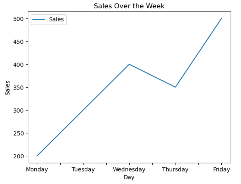
The real power of Pandas plotting lies in its versatility, which we can unlock with a slight tweak.

Hacked Version

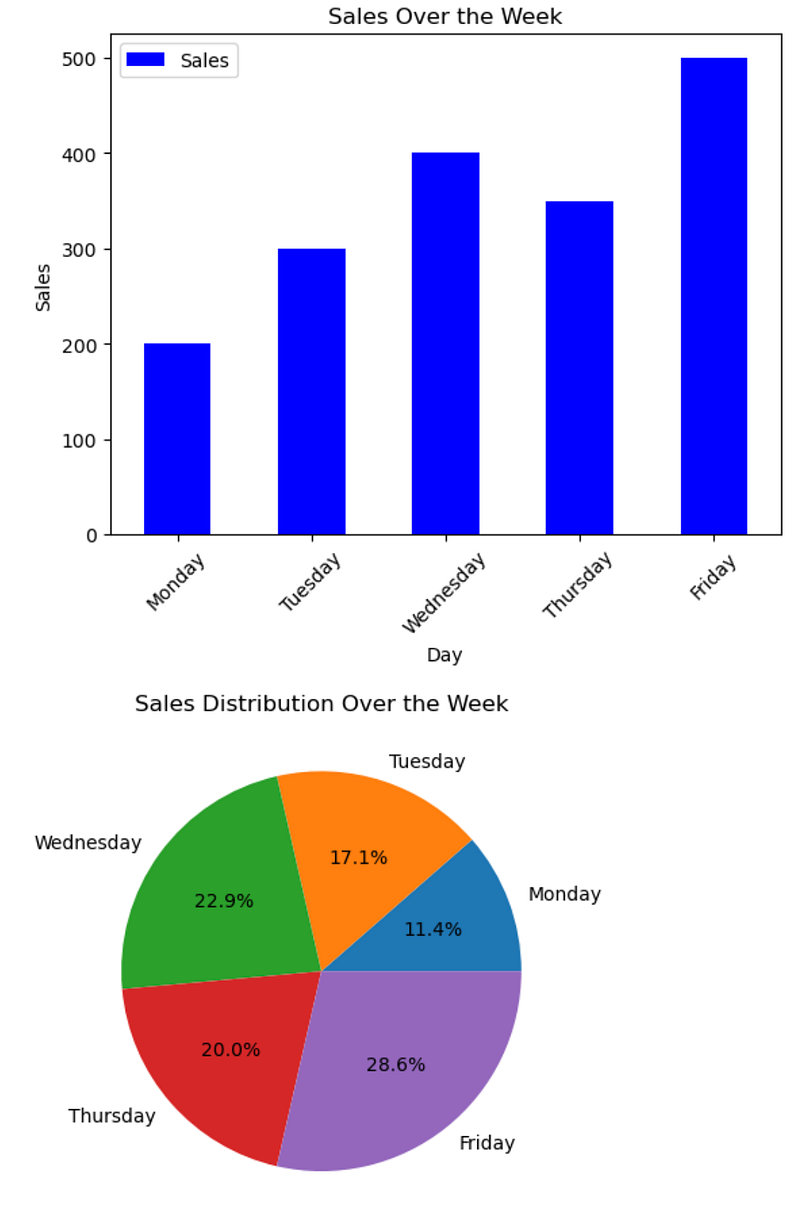
Utilizing Pandas Plotting with plot(kind='type') for Diverse Chart Types

Pandas’ .plot() function is highly customizable, with the kind parameter allowing you to easily switch between different plot types.

This enables the creation of a variety of visualizations without having to delve into the complexities of Matplotlib syntax for each type.

# Creating a bar chart
df.plot(kind='bar', x='Day', y='Sales', color='blue')
plt.title('Sales Over the Week')
plt.ylabel('Sales')
plt.xticks(rotation=45)  # Rotate labels to improve readability
plt.show()

# Creating a pie chart
df.set_index('Day')['Sales'].plot(kind='pie', autopct='%1.1f%%')
plt.ylabel('')  # Hide the y-label as it's unnecessary for pie charts
plt.title('Sales Distribution Over the Week')
plt.show()

Here is the output.

Optimizing DataFrames for Memory Efficiency

Working with large datasets in Pandas can be memory-intensive. By default, Pandas often allocate more memory than necessary for storing data types. Optimizing memory usage can significantly improve performance, especially when dealing with big data.

Normal Version

Regular DataFrame Usage

In standard practice, when we create or load a DataFrame, Pandas automatically determines the data types for each column. This automatic type assignment can lead to suboptimal memory usage:

import pandas as pd

# Sample data: Employee information
data = {
    'EmployeeID': [1, 2, 3, 4, 5],
    'Age': [28, 34, 45, 29, 40],
    'Salary': [50000, 60000, 80000, 55000, 75000]
}
df = pd.DataFrame(data)

# Check memory usage
df.info(memory_usage='deep')

Here is the output.

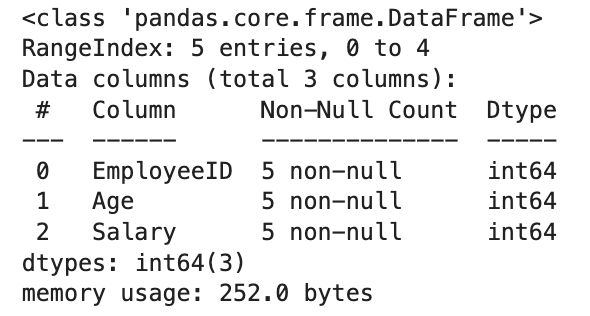
This will show the DataFrame’s memory usage, which can be more than necessary due to the default data types assigned.

Hacked Version

Applying astype() for Type Conversion and Memory Optimization

You can manually adjust the data types for each column using the astype() method, which allows for more memory-efficient storage types:

# Optimize by converting to more memory-efficient data types
optimized_df = df.copy()
optimized_df['EmployeeID'] = optimized_df['EmployeeID'].astype('int32')
optimized_df['Age'] = optimized_df['Age'].astype('int8')
optimized_df['Salary'] = optimized_df['Salary'].astype('int32')

# Check memory usage after optimization
optimized_df.info(memory_usage='deep')

Here is the output.

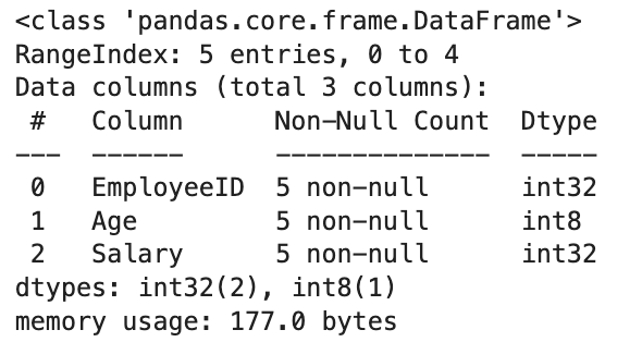
By converting to more memory-efficient data types (for example, using int8 for the 'Age' column, which only requires a range of 0 to 255), we can significantly reduce the memory footprint of our DataFrame.

For this simple example, we reduced the memory usage from 252 to 177 bytes, achieving a 29.76%. reduction.

This optimization is crucial for processing large datasets or when operating within memory-constrained environments.

Final Thoughts

In this article, we explored seven advanced Pandas techniques that are indispensable for AI experts, from simplifying data merges to optimizing memory usage for large datasets.

For more, you can subscribe to my Substack, where you can reach to;

#LearnAI : Helps you to learn AI with 7/24 available digital assistant (LearnAIWithMe GPT)
#JobHuntAI : Show AI tasks on Upwork, and show how it can be solved.
#Weekly AI Pulse: Will tune you AI news weekly.

Also you will be invited to our notion page, after becoming a paid subscriber, where you can reach links of our specialGPT’s, data projects, cheatsheets and more.

Here is the ChatGPT cheat sheet.

Here is my NumPy cheat sheet.

Here is the source code of the “How to be a Billionaire” data project.

Here is the source code of the “Classification Task with 6 Different Algorithms using Python” data project.

Here is the source code of the “Decision Tree in Energy Efficiency Analysis” data project.

Here is the source code of the “DataDrivenInvestor 2022 Articles Analysis” data project.

“Machine learning is the last invention that humanity will ever need to make.” Nick Bostrom