6 Statistical Terms I wish I knew before starting my first Data Science Job

As a data scientist, understanding statistical concepts is crucial to making informed decisions about data analysis and modelling. Unfortunately, crucial terms and techniques are often not covered in traditional academic coursework or training programs. This can leave new data scientists feeling unprepared for the complex and varied tasks they are expected to tackle in their first jobs. In this article, we will explore some of the critical statistical terms that I wish I had known before starting my first Data Science job. By the end of this article, you will have a better understanding of some of the essential statistical terms that every data scientist should know, which will help you to optimise your approach and avoid common pitfalls that can lead to inaccurate or unreliable results. Whether you’re just starting out in data science or looking to brush up on your statistical knowledge, I hope you’ll find this article helpful!

1. Bootstrapping

Bootstrapping is a statistical technique that involves resampling your data to generate multiple datasets for analysis. Instead of collecting new data, you use your existing data to create many new samples. This is done by randomly selecting data points from your original dataset with replacements, meaning that the same data point can be chosen more than once. For example, suppose you have a dataset of 100 observations and you want to estimate the mean of a variable. With bootstrapping, you would randomly select 100 observations from the dataset with replacement, compute the mean of those observations, and record it. You would then repeat this process many times, perhaps 1000 or more, to create a distribution of means. This distribution can then be used to estimate the standard error of the mean, construct confidence intervals, or perform hypothesis tests.

Bootstrapping is a useful technique when the assumptions of traditional statistical tests are not met or when your sample size is small. It can also be used to estimate the bias and variance of a model, compare different models, or validate the performance of a model. For example, suppose you want to compare the accuracy of two regression models for predicting house prices. With bootstrapping, you would randomly sample a subset of your data, fit each model to the subset, and record their performance. You would then repeat this process many times to generate distributions of the models’ performance. This can help you to understand the uncertainty in the models’ predictions and choose the better-performing model.

Here’s an example of how to perform bootstrapping in Python (using pandas and numpy)

import pandas as pd
import numpy as np

#Load Dataset (here we're crerating a sample dataframe)
df = pd.DataFrame({'numbers': [1, 2, 3, 4, 5, 6, 7, 8]})

# We define a function to compute the mean of a dataset
def mean_func(data):
    return np.mean(data)

# We set the number of bootstrap samples to 1000
n_bootstrap = 1000

#We generate bootstrap samples 
#by randomly selecting rows from 
#the original dataset with 
#replacement using the sample function

bootstrap_samples = []
for i in range(n_bootstrap):
    sample = df.sample(frac=1, replace=True)
    bootstrap_samples.append(sample)

# Compute means for each bootstrap sample
bootstrap_means = []
for sample in bootstrap_samples:
    mean = mean_func(sample)
    bootstrap_means.append(mean)

# Compute the 95% confidence interval 
# by calculating the 2.5th and 97.5th percentiles

alpha = 0.05
lower = np.percentile(bootstrap_means, alpha/2 * 100)
upper = np.percentile(bootstrap_means, (1 - alpha/2) * 100)

print(f"The mean is {np.mean(df)}")
print(f"The 95% confidence interval is [{lower}, {upper}]")

Output:

The mean is numbers    3.0

The 95% confidence interval is [1.8, 4.2]

In summary, bootstrapping is a powerful statistical technique that can help you to better understand the variability in your data and improve the accuracy and reliability of your analyses.

2. Student’s T-test

A t-test is a statistical test that allows you to compare the means of two groups of data and determine if they are significantly different. It helps you to answer questions such as: “Are the means of two groups of data different from each other?” or “Is the difference between two means statistically significant?”

There are two types of t-tests: the independent samples t-test and the paired samples t-test. The independent samples t-test is used when you have two independent groups of data, while the paired samples t-test is used when you have two related groups of data, such as pre-test and post-test measurements on the same subjects.

import pandas as pd
from scipy.stats import ttest_ind

# Load data into two separate dataframes
df1 = pd.read_csv('group1.csv')
df2 = pd.read_csv('group2.csv')

# Perform t-test
# using the ttest_ind function from the scipy.stats library
# The function returns the t-statistic and p-value of the test. 
t_stat, p_value = ttest_ind(df1['variable'], df2['variable'])

# Print results
print(f"t-statistic = {t_stat}")
print(f"p-value = {p_value}")

if p_value < 0.05:
    print("The means of the two groups are significantly different.")
else:
    print("There is no significant difference between the means of the two groups.")

The t-test is a useful statistical tool for comparing the means of two groups of data and determining if the difference between them is significant.

3. Effect Size

Effect size is the size of the difference between two groups or things. It measures the magnitude of the relationship or the degree of difference between the groups, independent of the sample size. Let’s say you have a big pile of cookies and your friend has a small pile of cookies. The effect size would be how many more cookies you have than your friend. If you have just a few more cookies than your friend, that’s a small effect size. But if you have a whole lot more cookies than your friend, that’s a big effect size. Effect size helps us understand how different things are from each other, so we can figure out if the difference is really important or not.

There are several ways to calculate the effect size, depending on the type of data and analysis used. Some common measures of effect size include Cohen’s d, Pearson’s r, and odds ratios.

import scipy.stats as stats
import numpy as np

# Create two groups of data
group1 = np.random.normal(10, 2, size=100)
group2 = np.random.normal(12, 2, size=100)

# Calculate Cohen's d
# which is the difference between the means 
# of the two groups divided by the pooled standard deviation. 
diff = group1.mean() - group2.mean()
pooled_std = np.sqrt((group1.std()**2 + group2.std()**2) / 2)
d = diff / pooled_std

# Print the results
print(f"Cohen's d: {d}")

How to interpret the output? A Cohen’s d of 0.2 is considered a small effect size (small difference or relationship between the groups), 0.5 is considered a medium effect size(moderate difference or relationship between the groups or variables), and 0.8 or higher is considered a large effect size (strong difference or relationship between the groups or variables).

The effect size is an important statistical concept that helps researchers to understand the practical significance of their findings and to compare results across different studies.

4. Power Analysis

Power analysis is a statistical method used to determine the sample size (how many data points/participants) required to detect a statistically significant effect in a study. It helps researchers to determine the probability of correctly rejecting the null hypothesis (i.e., finding a significant effect) if a true effect exists. At my job, we use it to estimate the number of participants for user research. In other words, power analysis allows researchers to estimate the statistical power of their study, which is the probability of detecting a true effect if it exists. A high statistical power means that the study is more likely to find a significant effect if there is one, while a low power means that the study is less likely to detect a significant effect even if there is one.

import statsmodels.stats.power as smp

# Set the parameters
effect_size = 0.5
alpha = 0.05 #or the p value
power = 0.8 #desired power level for the study

# Perform power analysis
# using statsmodel function
# passing in the effect size, alpha level, and power level 
nobs = smp.tt_ind_solve_power(effect_size=effect_size, alpha=alpha, power=power)

# Print the results
# which in this case would be 
# the sample size required to detect a medium-sized effect
print(f"Sample size required: {nobs}")

Output:

Sample size required: 63.765611775409525

So in this case we would need a sample size of around 64 to detect a medium-sized effect (effect size of 0.5) with an alpha level/p value of 0.05 and a power level of 0.8.

Power analysis is a crucial step in designing a study and determining the appropriate sample size to achieve the desired level of statistical power. It can help researchers to ensure that their study is well-powered and can detect significant effects if they exist.

5. Confidence Interval

A confidence interval is a range of values that is likely to contain the true value of a parameter or the true difference between two groups based on a sample of data. In other words, let’s say you’re interested in knowing the average height of all the people in your town. You can’t measure every single person, so you take a sample of citizens and calculate the sample mean height. However, you know that your sample mean is unlikely to be exactly equal to the true population mean (the actual average height of all the people in your town). A confidence interval gives you a range of values that likely contains the true population mean. For example, a 95% confidence interval means that if you repeated the sampling process many times, 95% of the time the true population mean would fall within the calculated interval. Confidence intervals are important because they help us understand the precision of our estimates. They also allow us to compare two groups and determine if the difference between them is statistically significant.

To calculate a confidence interval, we need to know the sample mean, sample standard deviation, sample size, and the level of confidence we want to use. We can use Python and the stats models package to calculate confidence intervals:

import numpy as np
import statsmodels.stats.api as sms

# Example data
data = np.array([2, 4, 6, 8, 10])


# Calculate 95% confidence interval for the mean
# The default level of confidence is 95%. 
ci = sms.DescrStatsW(data).tconfint_mean()

# Print the confidence interval
# The tconfint_mean function returns a tuple 
# containing the lower and upper bounds of the confidence interval.
print("95% Confidence interval:", ci)

Output:

95% Confidence interval: (2.3237900075540076, 9.676209992445992)

This means that if we repeated the sampling process many times, 95% of the time the true population mean would fall within the range of 2.32 to 9.68.

6. Central Limit Theorem

The central limit theorem (CLT) is a statistical concept which states that the distribution of sample means approaches a normal distribution as the sample size increases, regardless of the shape of the population distribution. In simpler terms, the central limit theorem tells us that if we take many random samples of the same size from any population, the means of those samples will be approximately normally distributed, even if the population itself is not normally distributed.

The practical use of the central limit theorem is that it allows us to make inferences about a population using a sample. Let’s revisit the height measurement example. If we want to estimate the average height of all people in your town, but it’s impossible to measure every citizen, we can take a random sample of citizens and calculate the sample mean. The central limit theorem tells us that if we take many random samples and calculate the sample mean, the distribution of those sample means will be approximately normal, and we can use this information to make statements about the population mean.

In Python, we can simulate the central limit theorem by generating random samples from a non-normal population distribution and calculating the sample means:

import numpy as np
import matplotlib.pyplot as plt


# Generate a non-normal population distribution
pop = np.random.uniform(0, 1, size=10000)

# Calculate the means of many random samples
# and store the sample means in a list
sample_means = []
for i in range(1000):
    sample = np.random.choice(pop, size=100)
    sample_mean = np.mean(sample)
    sample_means.append(sample_mean)

# Plot the distribution of sample means
plt.hist(sample_means, bins=30, density=True)
plt.xlabel("Sample mean")
plt.ylabel("Density")
plt.title("Central Limit Theorem")
plt.show()

Output:

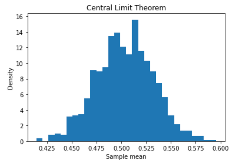
The resulting plot should show a roughly normal distribution of sample means, which demonstrates the central limit theorem.

Understanding these 6 statistical terms — effect size, power analysis, bootstrapping, t-test, confidence interval, and central limit theorem — can help you make better data-driven decisions, and ultimately improve your performance as a data scientist.

By no means is this an exhaustive list of statistical terms, it’s simply a list of terms which caught me off guard at my first DS job. As you continue to work with data, you’ll likely encounter many more statistical concepts that you’ll need to learn and apply.

With the help of Python and statistical libraries such as pandas, numpy, and scipy, you can easily apply these concepts to real-world data. So, take some time to explore these concepts and start applying them to your data analysis today!

Feel free to connect with me on LinkedIn.

Good luck with your Data Science journey! : )