
6 Reasons Why You Should Stop Using Histograms (and Which Plot You Should Use Instead)
Histograms are not free of biases. Actually, they are arbitrary and may lead to wrong conclusions about data. If you want to visualize a variable, better to choose a different plot.
Whether you are at a meeting with top executives or at a meetup with data-nerds, you can be sure of one thing: at some point, there will be a histogram.
And it’s not hard to see why. Histograms are incredibly intuitive: anyone understands them at a first glance. Moreover, they are an unbiased representation of the reality, right? Not so fast.
A histogram can be misleading and carry to faulty conclusions — even with simple data!
In this post, with the aid of some examples, we will go through 6 reasons why, when it comes to visualizing data, a histogram is hardly the best choice:
- It depends (too much) on the number of bins.
- It depends (too much) on variable’s maximum and minimum.
- It doesn’t allow to detect relevant values.
- It doesn’t allow to discern continuous from discrete variables.
- It makes it hard to compare distributions.
- It’s hard to make if you don’t have all the data in memory.
“Okay, I get it: histograms are not perfect. But do I have a choice?” Yes, you do!
In the end of the article, I will recommend a different plot — called CDP — that overcomes these flaws.
So, What’s Wrong With the Histogram?
1. It depends (too much) on the number of bins.
To draw a histogram, you must first decide the number of intervals, also called bins. There exist many different rules of thumb to do that (see this page for an overview). But how critical is this choice? Let’s take some real data and see how the histogram changes based on the number of bins.
The variable is the maximum heart rate (beats per minute) achieved by 303 people during some physical activity (data taken from the UCI heart disease dataset: source).
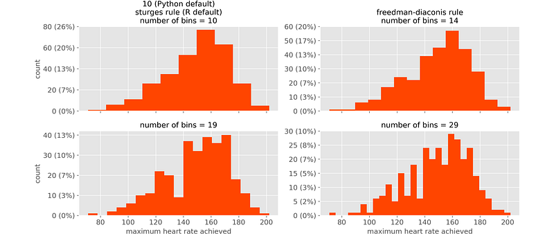
Looking at the upper left plot (which we would get by default in Python and R), we would have the impression of a nice distribution with a single peak (mode). However, if we looked at the other histograms, we would get a totally different picture. Histograms can lead to contradictory conclusions.
2. It depends (too much) on variable’s maximum and minimum.
Even once that the number of bins is set, intervals depend on the position of variable’s minimum and maximum. It’s enough that one of the two slightly changes, and all intervals change. In other words, histograms are not robust.
For instance, let’s try and change the variable’s maximum, while the number of bins is kept constant.
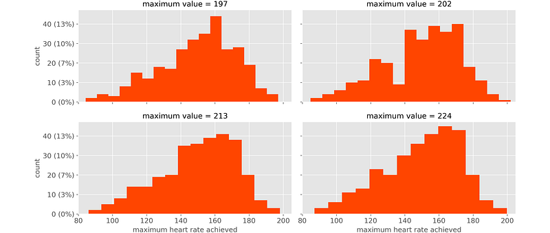
If a single value is different, the whole plot is different. This is an undesirable property, because we are interested in the overall distribution: a single value should make no difference!
3. It doesn’t allow to detect relevant values.
In general, when a variable contains some frequent values, we need to be aware of it. However, histograms don’t allow to do that, because they are based on intervals, and intervals “hide” individual values.
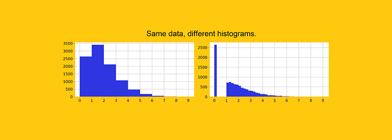
A classical example is when missing values are massively imputed to 0. For instance, let’s see a variable consisting of 10 thousand data-points, 26% of which are 0s.
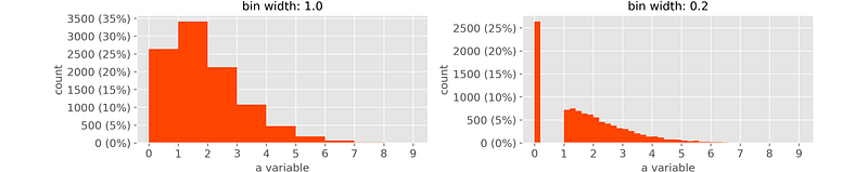
The plot on the left is what you get by default in Python. By looking at it, you would believe that this variable has a “smooth” behaviour and you wouldn’t even perceive that there’s a concentration of zeros.
The plot on the right is obtained by narrowing the bins, and gives a clearer representation of the reality. But the point is that, no matter how you narrow the bins, you will never be sure whether the first bin contains only 0s or some other values.
4. It doesn’t allow to discern continuous from discrete variables.
In general, we want to know whether a numeric variable is continuous or discrete. Given a histogram, it’s virtually impossible to tell that.
Let’s take variable “Age”. You may find Age = 49 years (when the age is truncated), or Age = 49.828884325804246 years (when the age is calculated as number of days since birth divided by 365.25). The first one is a discrete variable, whereas the second one is continuous.
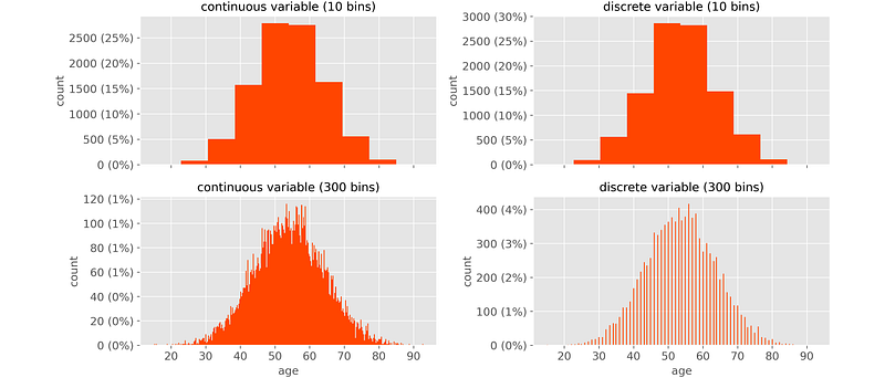
The one on the left is continuous, and the one on the right discrete. However, in the upper plots (Python’s default) you wouldn’t see any difference between the two: they look exactly the same.
5. It makes it hard to compare distributions.
It is often necessary to compare the same variable on different clusters. For instance, regarding UCI heart disease data above, we may want to compare:
- the whole population (as a reference)
- people younger than 50 & suffering from heart disease
- people younger than 50 & NOT suffering from heart disease
- people older than 60 & suffering from heart disease
- people older than 60 & NOT suffering from heart disease
This is what we would get:
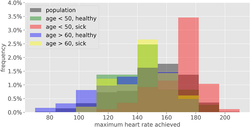
Histograms are based on areas and, when we try to make comparisons, the areas end up to be overlapped, making our job impossible.
6. It‘s hard to make if you don’t have all the data in memory.
If you have all the data in Excel, R or Python, it’s easy to make a histogram: in Excel you just need to click on the histogram’s icon, in R to execute the command hist(x), and in Python plt.hist(x).
But suppose that your data are stored in a database. You don’t want to download all the data just to make a histogram, right? Basically, all you need is a table containing, for each bin, the extremes of the interval and the count of observations. Something like this:
| INTERVAL_LEFT | INTERVAL_RIGHT | COUNT         |
|---------------|----------------|---------------|
| 75.0          | 87.0           | 31            |
| 87.0          | 99.0           | 52            |
| 99.0          | 111.0          | 76            |
| ...           | ...            | ...           |
But obtaining it through a SQL query is not as straightforward as it seems. For example, in Google’s Big Query, the code would be:
WITHSTATS AS (
SELECT
COUNT(*) AS N,
APPROX_QUANTILES(VARIABLE_NAME, 4) AS QUARTILES
FROM
TABLE_NAME
),BIN_WIDTH AS (
SELECT
-- freedman-diaconis formula for calculating the bin width
(QUARTILES[OFFSET(4)] — QUARTILES[OFFSET(0)]) / ROUND((QUARTILES[OFFSET(4)] — QUARTILES[OFFSET(0)]) / (2 * (QUARTILES[OFFSET(3)] — QUARTILES[OFFSET(1)]) / POW(N, 1/3)) + .5) AS FD
FROM
STATS
),HIST AS (
SELECT
FLOOR((TABLE_NAME.VARIABLE_NAME — STATS.QUARTILES[OFFSET(0)]) / BIN_WIDTH.FD) AS INTERVAL_ID,
COUNT(*) AS COUNT
FROM
TABLE_NAME,
STATS,
BIN_WIDTH
GROUP BY
1
)SELECT
STATS.QUARTILES[OFFSET(0)] + BIN_WIDTH.FD * HIST.INTERVAL_ID AS INTERVAL_LEFT,
STATS.QUARTILES[OFFSET(0)] + BIN_WIDTH.FD * (HIST.INTERVAL_ID + 1) AS INTERVAL_RIGHT,
HIST.COUNT
FROM
HIST,
STATS,
BIN_WIDTHA bit cumbersome, isn’t it?
An Alternative: the Cumulative Distribution Plot
After seeing 6 reasons why a histogram is not the ideal choice, a natural question is: “Do I have any alternative?” Good news: a better alternative does exist, and is called “Cumulative Distribution Plot” (CDP). I know the name isn’t quite as memorable, but I promise it’s worth it.
A Cumulative Distribution Plot is a plot of the quantiles of a variable. In other words, each point on the CDP shows:
- on the x-axis: the original value of the variable (as happens with the histogram);
- on the y-axis: how many observations have the same value or less.
Let’s see an example on the usual variable: maximum heart rate.
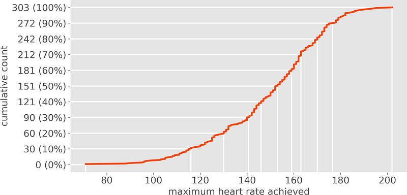
Let’s take the point with coordinates x = 140 and y = 90 (30%). On the horizontal axis you see the variable’s value: 140 heart beats per minute. On the vertical axis you see the count of observations that have a heart rate equal or lower than 140 (in this case 90 people, which means 30% of the sample). Therefore, 30% of our sample have 140 or less heart beats per minute.
What’s the point of a plot telling you how many observations are “equal or lower” than a given level ? Why not just “equal”? Because, otherwise, the outcome would depend on the single values of the variable. And this wouldn’t work, because each value has very few observations (usually just one, if the variable is continuous). On the contrary, CDPs rely on quantiles, which are more stable, meaningful and easy to read.
Additionally, CDP is much more useful. If you think about it, you often need to answer questions such as “how many are between 140 and 160?”, or “how many are above 180?”. Having a CDP under your nose, you can give an immediate answer. With a histogram, this would be impossible.
The CDP solves all the issues that we have seen above. In fact, compared to a histogram:
1. It doesn’t require any user choice. Given some data, there is only one possible CDP.
2. It doesn’t suffer from outliers. Extreme values have no effect on a CDP, since the quantiles don’t change.
3. It allows to detect relevant values. If there exists a concentration of data-points on some specific value it’s immediately evident, since there will be a vertical segment into correspondance of the value.
4. It allows to recognize a discrete variable at first glance. If there exists just a bunch of possible values (i.e. the variable is discrete) it’s immediately evident, since the curve is staircase-shaped.
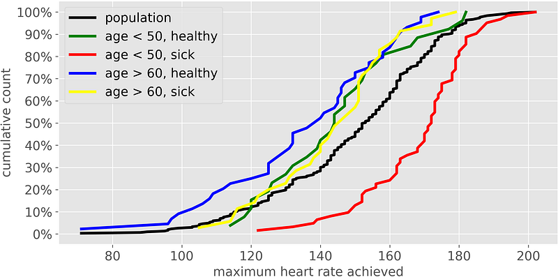
5. It makes it easy to compare distributions. It’s easy to compare two or more distributions on the same plot, since they are just curves, not areas. Moreover, the y-axis always ranges between 0 and 100%, making the comparison even more straightforward. For instance, this is the example that we have seen above:
6. It’s easy to make also if you don’t have all the data in memory. All you need are quantiles, which can be obtained effortlessly in SQL:
SELECT
  COUNT(*) AS N,
  APPROX_QUANTILES(VARIABLE_NAME, 100) AS PERCENTILES
FROM
  TABLE_NAME
How to Make a Cumulative Distribution Plot in Excel, R, Python
In Excel, you need to build two columns. The first one with 101 numbers equally distributed from 0 to 1. The second column should contain the percentiles which can be obtained through the formula: =PERCENTILE(DATA, FRAC), where DATA is the vector containing data and FRAC is the first column: 0.00, 0.01, 0.02, 0.03, …, 0.98, 0.99, 1. Then, you just have to plot the two columns, taking care of putting the variable’s values on the x-axis.
In R, it’s as simple as:
plot(ecdf(data))In Python:
from statsmodels.distributions.empirical_distribution import ECDF
import matplotlib.pyplot as plt
ecdf = ECDF(data)
plt.plot(ecdf.x, ecdf.y)Thank you for reading!
If you find my work useful, you can subscribe to get an email every time that I publish a new article (usually once a month).
If you want to support my work, you can buy me a coffee.
If you’d like, add me on Linkedin!


