
6 Pandas tricks you should know to speed up your data analysis
Some of the most helpful Pandas tricks

In this article, you’ll learn some of the most helpful Pandas tricks to speed up your data analysis.
- Select columns by data types
- Convert strings to numbers
- Detect and handle missing values
- Convert a continuous numerical feature into a categorical feature
- Create a DataFrame from the clipboard
- Build a DataFrame from multiple files
Please check out my Github repo for the source code.
1. Select columns by data types
Here are the data types of the Titanic DataFrame
df.dtypesPassengerId int64
Survived int64
Pclass int64
Name object
Sex object
Age float64
SibSp int64
Parch int64
Ticket object
Fare float64
Cabin object
Embarked object
dtype: objectLet’s say you need to select the numeric columns.
df.select_dtypes(include='number').head()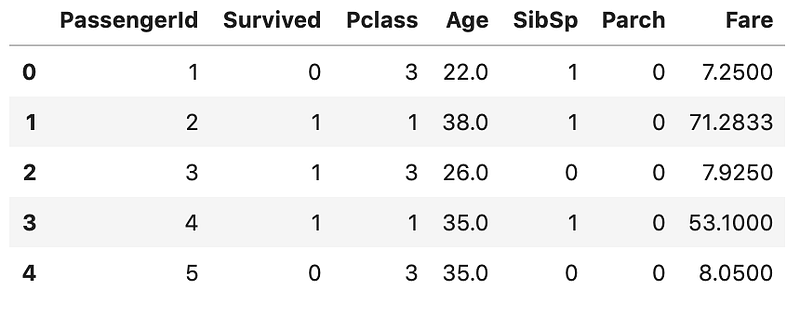
This includes both int and float columns. You could also use this method to
- select just object columns
- select multiple data types
- exclude certain data types
# select just object columns
df.select_dtypes(include='object')
# select multiple data types
df.select_dtypes(include=['int', 'datetime', 'object'])# exclude certain data types
df.select_dtypes(exclude='int')2. Convert strings to numbers
There are two methods to convert a string into numbers in Pandas:
- the
astype()method - the
to_numeric()method
Let’s create an example DataFrame to have a look at the difference.
df = pd.DataFrame({ 'product': ['A','B','C','D'],
                   'price': ['10','20','30','40'],
                   'sales': ['20','-','60','-']
                  })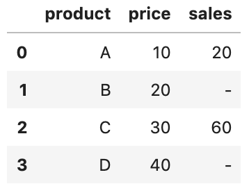
The price and sales columns are stored as strings and so result in object columns:
df.dtypesproduct object
price object
sales object
dtype: objectWe can use the first method astype() to perform the conversion on the price column as follows
# Use Python type
df['price'] = df['price'].astype(int)
# alternatively, pass { col: dtype }
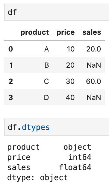
df = df.astype({'price': 'int'})However, this would have resulted in an error if we tried to use it on the sales column. To fix that, we can use to_numeric() with argument errors='coerce'
df['sales'] = pd.to_numeric(df['sales'], errors='coerce')Now, invalid values - get converted into NaN and the data type is float.
3. Detect and handle missing values
One way to detect missing values is by using info() method and take a look at the column Non-Null Count.
df.info()RangeIndex: 891 entries, 0 to 890
Data columns (total 12 columns):
# Column Non-Null Count Dtype
--- ------ -------------- -----
0 PassengerId 891 non-null int64
1 Survived 891 non-null int64
2 Pclass 891 non-null int64
3 Name 891 non-null object
4 Sex 891 non-null object
5 Age 714 non-null float64
6 SibSp 891 non-null int64
7 Parch 891 non-null int64
8 Ticket 891 non-null object
9 Fare 891 non-null float64
10 Cabin 204 non-null object
11 Embarked 889 non-null object
dtypes: float64(2), int64(5), object(5)
memory usage: 83.7+ KBWhen the dataset is large, we can count the number of missing values instead. df.isnull().sum() returns the number of missing values for each column
df.isnull().sum()PassengerId 0
Survived 0
Pclass 0
Name 0
Sex 0
Age 177
SibSp 0
Parch 0
Ticket 0
Fare 0
Cabin 687
Embarked 2
dtype: int64df.isnull().sum().sum() returns the total number of missing values.
df.isnull().sum().sum()886
In addition, we can also find out the percentage of values that are missing by running df.isna().mean()
ufo.isna().mean()PassengerId 0.000000
Survived 0.000000
Pclass 0.000000
Name 0.000000
Sex 0.000000
Age 0.198653
SibSp 0.000000
Parch 0.000000
Ticket 0.000000
Fare 0.000000
Cabin 0.771044
Embarked 0.002245
dtype: float64Dropping missing values
To drop rows if any NaN values are present
df.dropna(axis = 0)To drop columns if any NaN values are present
df.dropna(axis = 1)To drop columns in which more than 10% of values are missing
df.dropna(thresh=len(df)*0.9, axis=1)Replacing missing values
To replace all NaN values with a scalar
df.fillna(value=10)To replace NaN values with the values in the previous row.
df.fillna(axis=0, method='ffill')To replace NaN values with the values in the previous column.
df.fillna(axis=1, method='ffill')The same, you can also replace NaN values with the values in the next row or column.
# Replace with the values in the next row
df.fillna(axis=0, method='bfill')
# Replace with the values in the next column
df.fillna(axis=1, method='bfill')The other common replacement is to replace NaN values with the mean. For example to replace NaN values in column Age with the mean.
df['Age'].fillna(value=df['Age'].mean(), inplace=True)For more about missing values in Pandas, please check out Working with missing values in Pandas.
4. Convert a continuous numerical feature into a categorical feature
In the step of data preparation, it is quite common to combine or transform existing features to create a more useful one. One of the most popular ways is to create a categorical feature from a continuous numerical feature.
Let’s take a look at the Age column from the Titanic dataset
df['Age'].head(8)0 22.0
1 38.0
2 26.0
3 35.0
4 35.0
5 NaN
6 54.0
7 2.0
Name: Age, dtype: float64Age is a continuous numerical attribute, but what if you want to convert it into a categorical attribute, for example, convert ages to groups of age ranges: ≤12, Teen (≤18), Adult (≤60), and Older (>60)
The best way to do this is by using the Pandas cut() function:
import sysdf['ageGroup']=pd.cut(
df['Age'],
bins=[0, 13, 19, 61, sys.maxsize],
labels=['<12', 'Teen', 'Adult', 'Older']
)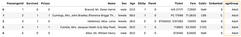
And calling head() on the ageGroup column should also display the column information.
df['ageGroup'].head(8)0 Adult
1 Adult
2 Adult
3 Adult
4 Adult
5 NaN
6 Adult
7 <12
Name: ageGroup, dtype: category
Categories (4, object): [<12 < Teen < Adult < Older]5. Create a DataFrame from the clipboard
Pandas read_clipboard() function is a very handy way to get data into a DataFrame as quickly as possible.
Suppose we have the following data and we want to create a data frame from it:
     product   price
0    A         10
1    B         20
2    C         30
4    D         40
We just need to select the data and copy it to the clipboard. Then, we can use the function to read it into a DataFrame.
df = pd.read_clipboard()
df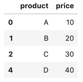
6. Build a DataFrame from multiple files
Your dataset might spread across multiple files, but you want to read the dataset into a single DataFrame.
One way to this is to read each file into its own DataFrame, combine them together, and then delete the original DataFrame, but that would be memory inefficient.
A better solution is to use the built-in glob module (Thanks to Data School Pandas Tricks).
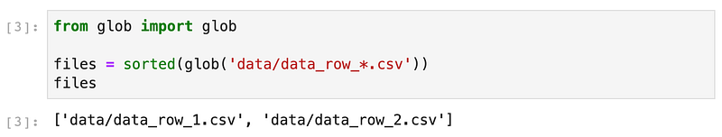
In this case, glob() is looking in the data directory for all CSV files that begin with the word “data_row_”. glob() returns filenames in an arbitrary order, which is why we sorted the list using sort() the function.
For row-wise data
Let’s say that our dataset is spread across 2 files, data_row_1.csv and data_row_2.csv, in row-wise
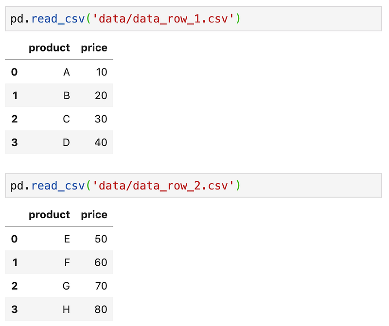
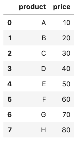
To create a DataFrame from the 2 files.
files = sorted(glob('data/data_row_*.csv'))
pd.concat((pd.read_csv(file) for file in files), ignore_index=True)sorted(glob('data/data_row_*.csv')) returns filenames. After that, we read each of the files using read_csv() and pass the results to the concat() function, which will concatenate the rows into a single DataFrame. In addition, to avoid duplicate value in the index, we tell the concat() to ignore the index (ignore_index=True) and instead use the default integer index.
For column-wise data
Let’s say that our dataset is spread across 2 files, data_col_1.csv and data_col_2.csv, in column-wise.
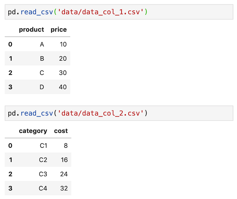
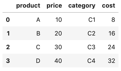
To create a DataFrame from the 2 files.
files = sorted(glob('data/data_col_*.csv'))
pd.concat((pd.read_csv(file) for file in files), axis=1)
This time, we tell the concat() function to concatenate along the columns axis.
That’s it
Thanks for reading.
Please checkout the notebook on my Github for the source code.
Stay tuned if you are interested in the practical aspect of machine learning.


