Temporal Fusion Transformer: Time Series Forecasting with Interpretability

Google’s state-of-the-art Transformer has it all

Preliminaries

First and foremost, let’s be clear: The era of tailoring a model to a single time series, either univariate or multivariate, is long gone.

Nowadays, in the big data era, the creation of new data points is extremely cheap. Imagine a large electrical company having thousands of sensors that measure the power consumption of different entities (e.g. households, factories) or an investment portfolio with a large number of stocks, mutual funds, bonds and so on. In other words, time series could be multivariate, with different distributions and could be accompanied by additional exploratory variables. And of course don’t forget the usual suspects: missing data, trend, seasonality, volatility, drift and rare events! In order to create a competitive model in terms of forecasting power, all variables should be factored in, apart from historical data.

Let’s take a step back and rethink what specifications a state-of-the-art, time series model should take into consideration:

1. Obviously, the model should be applied on either single or multidimensional sequences.
2. The model should account for multiple time series, ideally thousands of them. Do not confuse this with multivariate time series. It means time series with different distributions, trained on a single model.
3. Apart from temporal data, the model should be able to use historical information which is unknown in the future. For example, if we are to create a model that forecasts air pollution level, we would like to be able to use humidity as an external time series, which is known only up to present time. For example, all autoregressive methods (e.g. ARIMA models) including Amazon’s DeepAR[1] suffer from this limitation.
4. External static variables which are non-temporal should also be taken into account. For example, weather forecasting in different cities (city is the static variable).
5. The model should be extremely adaptive. Time sequences can be fairly complex or noisy, while others can be simply modeled with seasonal naive predictors. Ideally, the model should be able to differentiate these cases.
6. Multi-step prediction functionality is also a must. One-step ahead prediction models which recursively feed predictions could also work. However, keep in mind that for long range predictions the errors start to rack up.
7. In many cases, a simple prediction of the target variable is not enough. The algorithm should be able to output prediction intervals as well, which reflect the prediction uncertainty.
8. The ideal model is easy to use and can be deployed seamlessly in a production environment.
9. Last but not least, the past few years ‘black box models’ have started losing popularity. Explainability has now become a top priority, especially in production. In some cases, explainability is favored over accuracy.

Note: For a hands-on project on Temporal Fusion Transformer, check this article. Also, check my list of the Best Deep Learning Forecasting Models.

Enter Temporal Fusion Transformer (TFT)

What Is A Temporal Fusion Transformer? Temporal Fusion Transformer (TFT) is an attention-based Deep Neural Network, optimized for great performance and interpretability. Before delving into the specifics of this cool architecture, we briefly describe its advantages and novelties :

1. Rich features: TFT supports 3 types of features: i) temporal data with known inputs into the future ii) temporal data known only up to the present and iii) exogenous categorical/static variables, also known as time-invariant features.
2. Heterogeneous time series: Supports training on multiple time series, coming from different distributions. To achieve that, the TFT architecture splits processing into 2 parts: local processing which focuses on the characteristics of specific events and global processing which captures the collective characteristics of all time series.
3. Multi-horizon forecasting: Supports multi-step predictions. Apart from the actual prediction, TFT also outputs prediction intervals, by using the quantile loss function.
4. Interpretability: At its core, TFT is a transformer-based architecture. By taking advantage of self-attention, this model presents a novel Muti Head attention mechanism which when analyzed, provides extra insight on feature importances. For example, Multi-Horizon Quantile Recurrent Forecaster (MQRNN)[3] is another DNN implementation with good performance but does not provide any insight regarding feature interpretability.
5. High Performance: During benchmarks, TFT outperformed traditional statistical models (ARIMA) as well as DNN-based models such as DeepAR, MQRNN and Deep Space-State Models (DSSM)[4].
6. Documentation: Although it is a relatively new model, there are already open source implementations of TFT both in Tensorflow and Python.

Figure 1 shows the top-level architecture of Temporal Fusion Transformer:

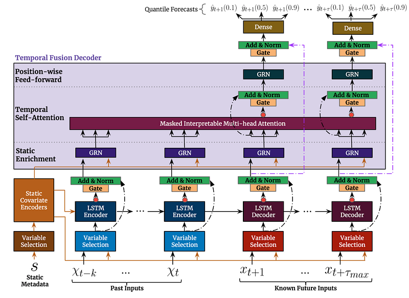
While this image may look intimidating, the model is actually quite easy to understand.

For a given timestep t , a lookback window k , and a τmax step ahead window, where t⋹ [t-k..t+τmax], the model takes as input: i) Observed past inputs x in the time period [t-k..t], future known inputs x in the time period [t+1..t+τmax] and a set of static variables s (if exist). The target variable y also spans the time window [t+1..t+τmax].

Next, we are going to describe step-by-step all the individual components and how they work together.

Gated Residual Network (GRN)

Figure 2 shows a component proposed by the paper, called Gated Residual Network (GRN), which is used as a basic block numerous time throughout TFT. The key points for this network are the following:

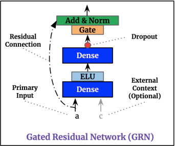
• It has two dense layers and two types of activation functions called ELU (Exponential Linear Unit) and GLU (Gated Linear Units). GLU was first used in the Gated Convolutional Networks [5] architecture for selecting the most important features for predicting the next word. In fact, both of these activation functions help the network understand which input transformations are simple and which require more complex modeling.
• The final output passes through standard Layer Normalization. The GRN also contain a residual connection, meaning that the network could learn, if necessary, to skip the input entirely. In some cases, depending where the GRN is situated, the network can also make use of static variables.

Variable Selection Network (VSN)

This component is shown in Figure 3. As its name implies, it functions as a feature selection mechanism. Remember what we said earlier: Not all time series are complex. The model should be able to distinguish insightful features from the noisy ones. Also, since there are 3 types of inputs, TFT uses 3 instances of the Variable Selection Network. Thus, each instance has different weights (notice the different colors of each VSN unit in Figure 1).

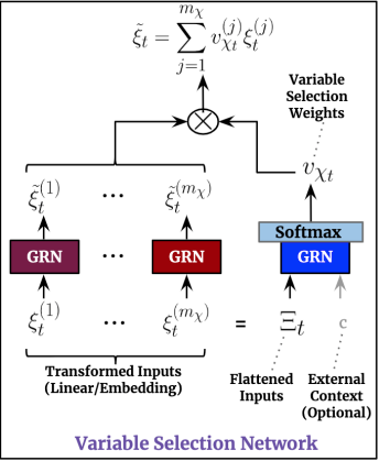
Naturally, the VSN utilizes GRN under the hood for its filtering capabilities. This is how it works:

• At time t the flattened vector of all past inputs (called Ξ_t) of the corresponding lookback period is fed through a GRN unit (in blue) and then a softmax function, producing a normalized vector of weights u.
• Moreover, each feature passes through its own GRN, which leads to the creation of a processed vector called ξ_t, one for every variable.
• Finally, an output is calculated as a linear combination of ξ_t and u.
• Note that the each feature has its own GRN, but the GRN for each feature is the same across all time steps during the same lookback period.
• The VSN for static variables does not take into account the context vector c

LSTM Encoder Decoder Layer

The LSTM Encoder Decoder Layer is part of many implementations, especially in NLP. It is displayed in Figure 1. This component serves two purposes:

Up to this point, the input has passed through VSN and has properly encoded and weighted the features. However, since our input is time-series data, the model should also make sense of the time/sequential ordering. Consequently, the first goal of the LSTM Encoder Decoder module is to produce context-aware embeddings, which are called φ. This is similar to the positional encoding used in the classic Transformer where we add sine and cosine signals. But why the authors choose the LSTM Encoder Decoder instead?

Because the model should account for all types of input. The known past inputs are fed into the encoder, while the known future inputs are fed into the decoder. And what about the static information? Is it possible to just merge the context aware embeddings produced by LSTM Encoder Decoder with the context vectors c of static variables?

Unfortunately, this would be inaccurate because we will mix temporal with static information. The correct way to do this is by applying a method used by [6] that correctly conditions the input based on exogenous data: Specifically, instead of setting the initial h_0 hidden state as well as the cell state c_0of the LSTM to 0, they are initialized with the c_h and c_c vectors respectively (which are produced from the static covariate encoder of TFT). As a consequence, the final context-aware embeddings φ will be properly conditioned on the exogenous information, without altering the temporal dynamics.

Interpretable Multi-Head Attention

This is the last part of the TFT architecture. In this step, the familiar self-attention mechanism[7] is applied which helps the model learn long range dependencies across different time steps.

All Transformer-based architectures leverage Attention to learn complex dependencies among the input data. If you are not familiar with the Attention-based implementations, check this source[8] (this is the best online source for understanding the Transformer model).

Temporal Fusion Transformer proposes a novel interpretable Multi-Head Attention mechanism, which contrary to the standard implementation, provides feature interpretability. In the original architecture there are different ‘heads’ (Query/Key/Value weight matrices) in order to to project the input into different representation subspaces. The drawback of this approach is that the weight matrices have no common ground and thus cannot be interpreted. TFT’s multi-head attention adds a new matrix/grouping such that the different heads share some weights which then can be interpreted in terms seasonality analysis.

Quantile Regression

In numerous applications where time series forecasting is involved, the prediction of the target variable is not enough. It is equally important to estimate the uncertainty of the prediction(s). Usually, this comes in the form of prediction intervals. Should we decide to include prediction intervals in the output, linear regression and the mean square error become inapplicable.

Standard linear regression uses the method of ordinary least squares (OLS) to calculate the conditional mean of the target variable across different values of the features. Prediction intervals from the OLS solution are based on the assumption that the residuals have constant variance, which is not always the case. On the other hand, quantile regression, which is an extension of Standard linear regression, estimates the conditional median of the target variable and can be used when assumptions of linear regression are not met. Apart from the median, quantile regression can also calculate the 0.25 and 0.75 quantiles (or any percentile for that matter) which means the model has the ability to output a prediction interval around the actual prediction. Figure 4 shows an example of how quantiles/percentiles look like in a regression problem:

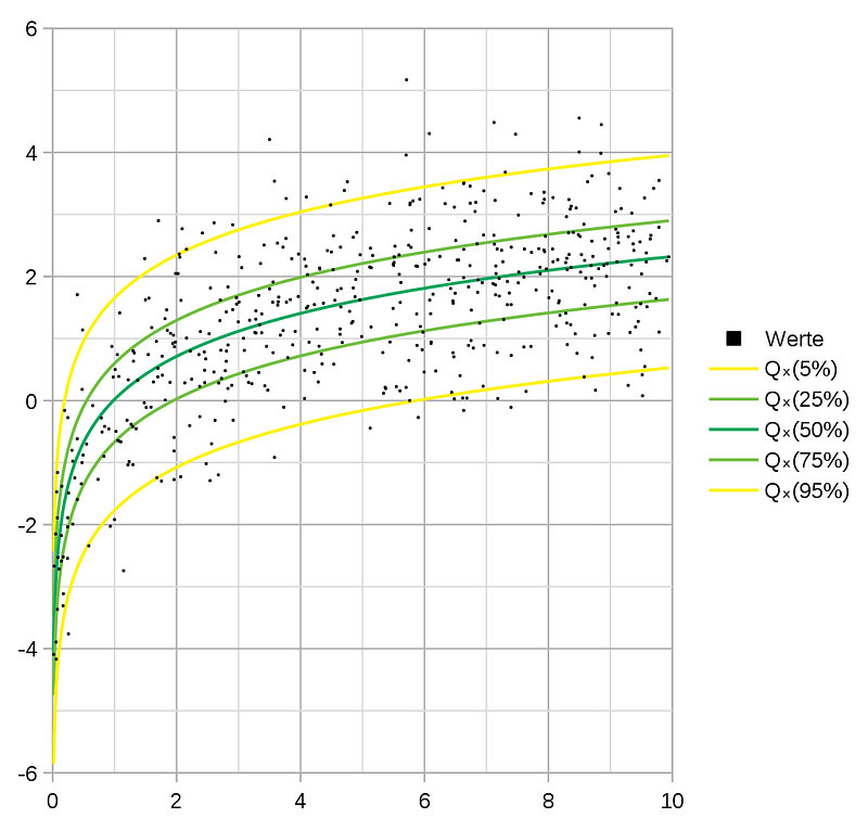
Given y and ŷ the actual value and the prediction respectively, and q a value for the quantile between 0 and 1, the quantile loss function is defined as:

As the value of q increases, overestimations are penalized by a larger factor compared to underestimations. For instance, for q equal to 0.75, overestimations will be penalized by a factor of 0.75, and underestimations by a factor of 0.25. That’s how the prediction intervals are created.

The Temporal Fusion Transformer implementation is trained by minimizing the quantile loss summed across q ⋹ [0.1, 0.5, 0.9]. This is done for benchmarking purposes, in order to match the experimental configuration used by other popular models. Also, it goes without saying that the use of quantile loss is not exclusive -other types of loss functions can be used such MSE, MAPE and so on.

Python Implementation

In the original paper, the Temporal Fusion Transformer model is compared against other popular time series models such as DeepAR, ARIMA and so on. Some of the datasets which the authors use for benchmarking are:

• Electricity Load Diagrams Dataset (UCI) [9]
• PEM-SF Traffic Dataset (UCI) [9]
• Favorita Grocery Sales (Kaggle) [10]

For more information about which configurations/hyperparameters are used for each dataset, check the original paper[2].

During benchmarks, TFT outperformed traditional statistical models (ARIMA) as well as DNN-based models such as DeepAR, MQRNN and Deep Space-State Models (DSSM)

Also, the authors kindly provide an open-source implementation of TFT in Tensorflow 1.x along with the corresponding hyperparameter configuration regarding each dataset for reproducibility purposes. Moreover, you can also find a modified version for Tensorflow 2.x here.

Let’s create a minimum working example using the Electricity Load Diagrams Dataset, which we will refer to as electricity for short . This dataset contains the electrical consumption (in kW) of 370 consumers. The datapoints are sampled every 15 minutes. Before proceeding to forecasting, the dataset is first preprocessed:

1. Time granularity becomes hourly.
2. Using the date information, we create the following (numerical) features: hour, day of week, and hours from start.
3. The categorical_id is an id for each consumer.
4. The target variable is power_usage.
5. The dataset is split into train, validation and test sets.
6. The train dataset is normalized. Specifically, numerical variables (including the target variable) are standardized(z-normalization) and the single categorical feature is label-encoded. It is imperative to understand that normalization takes place separately for each time-series/consumer, because time-sequences have different characteristics (mean and variance). Scalers are also kept for reverting predictions back to their original values.

The goal is to forecast the power usage of the next day(1*24 hours), by using the past week (7*24 hours).

For this example, we will use the updated version of TFT for Tensorflow 2.x. You could quickly setup a minimum working example in Conda:

Tensorflow 2.x.

# Download TFT. Kudos to greatwhiz for making TFT compatible to TF # 2.x!
!git clone https://github.com/greatwhiz/tft_tf2.git

# Install any missing libraries in Conda environment
!pip install pyunpack
!pip install wget

The implementation also contains scripts for downloading and preprocessing the aforementioned datasets: For the electricity dataset, execute:

# The structure of the command is:
# python3 -m script_download_data $EXPT $OUTPUT_FOLDER

!python3 tft_tf2/script_download_data.py electricity electricity_dataset

where electricity_dataset is the folder where the preprocessed data will be stored. This is what the preprocessed dataset looks like:

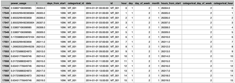
Not all of these variables are considered for training though. The model will make use of the variables which we discussed above.

Finally, execute the training script:

# The structure of the command is:
# python3 -m script_train_fixed_params $EXPT $OUTPUT_FOLDER $USE_GPU

!python3 tft_tf2/script_train_fixed_params.py electricity electricity_dataset ‘yes’

By default, this script runs in testing mode, which means the model will train for only 1 epoch and use only 100 and 10 training and validation instances respectively. To initiate a complete training with the optimal hyperparameters found in the original paper, in the script_train_fixed_params.py set use_testing_mode=True. For a complete training, the model will take approximately 7–8 hours on Colab with GPU enabled.

Pytorch

Temporal Fusion Transformer is also available in PyTorch. Check this comprehensive tutorial for more info.

Explainability

One of the strongest points regarding Temporal Fusion Transformer is explainability. In the context of a time series problem, explainability makes sense in many situations.

Feature-Wise

First of all, Temporal Fusion Transformer attempts to calculate the impact of each feature by taking into account the robustness of predictions. Feature importance can be measured by analyzing the weights u of all Variable Selection Network modules across the entire test set. For the Electricity dataset in Table 1 we have:

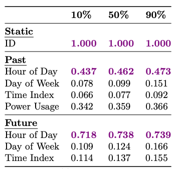
All feature scores take values between 0 and 1. The ID variable plays a major role since it distinguishes one time-series from another. Next is Hour of Day, which is expected since power consumption follows specific patterns throughout the day.

Seasonality

Using the interpretable Multi-Head Attention layer, we can take it one step further and calculate the ‘persistent temporal patterns’. More specifically, the attention weights from this layer can reveal which time-steps during the lookback period are the most important. As a consequence, visualization of those weights reveals the most prominent seasonalities. For instance, in Figure 5 we have:

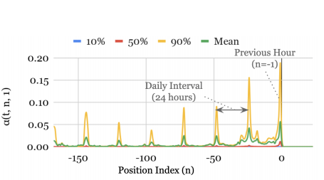
where a(t,n,1) is the attention score for horizon equal to 1 (same as one-step ahead) and n⋹[-(7*24)..0]. In other words, the plot clearly displays that the dataset exhibits a daily seasonal pattern.

Closing Remarks

To sum up, Temporal Fusion Transformer is a versatile model with high performance. The architecture of Temporal Fusion Transformer has incorporated numerous key advancements from the Deep Learning domain, while at the same time proposes some novelties of its own. The most fundamental of its features however is the ability to provide interpretable insights in terms of forecasting. Besides, this is one of the directions where Deep Learning is headed in the future, according to Gartner.

Thank you for reading!

• Subscribe to my newsletter!
• Follow me on Linkedin!

References

[1] D. Salinas et al., DeepAR: Probabilistic forecasting with autoregressive recurrent networks, International Journal of Forecasting (2019).

[2] Bryan Lim et al., Temporal Fusion Transformers for Interpretable Multi-horizon Time Series Forecasting, September 2020

[3] R. Wen et al., A Multi-Horizon Quantile Recurrent Forecaster, NIPS, 2017

[4] S. S. Rangapuram, et al., Deep state space models for time series forecasting, NIPS, 2018.

[5] Y. Dauphin et al., Language modeling with gated convolutional networks, ICML, 2017

[6] Andrej Karpathy, Li Fei-Fei, Deep Visual-Semantic Alignments for Generating Image Descriptions

[7] A. Vaswani et al. Attention Is All You Need, Jun 2017

[8] J. Alammar, The Illustrated Transformer

[9] Dua, D. and Graff, C. (2019). UCI Machine Learning Repository . Irvine, CA: University of California, School of Information and Computer Science.

[10] Favorita Grocery Sales Forecasting, Kaggle, Licence CC0: Public Domain