Getting started with F1 statistics and Python

Data preparation in Python for the analysis of F1 statistics with the Ergast dataset.

This tutorial describes how to use historic Formula One data for analysis. It covers obtaining the data, cleaning the data and two first analyses made with this data (more will follow!). The main focus in this article is the data preparation of this data set for analysis. It may feel as the dirty work, but good data preparation pays itself back. Easy.

The data is retrieved from the Ergast Developer API. This is an API providing historical data on F1 races, starting in 1950, though not all data is complete. Data is available up to the current season, containing all planned races and results for all completed races.

The available data contains the following table:

Drivers — Information on all current and previous drivers
Constructors — Information on all current and previous constructors
Race results, both constructor and driver
Qualifying results — Results of all qualifying sessions, including the seperate Q1, A2 and Q3 sessions.
Lap times — Lap times of all completed laps by all drivers in all events
Pit stops — All pit stops made, when and duration (pit in — pit out)
Standings, both constructor and driver after each race

There are two ways to access the data. First, there is a REST API to retrieve information from the data set. Using specific URL GET-request, e.g. http://ergast.com/api/f1/2008/8/results returns the results of the 8th race in the 2008 season.

Second, it is possible to directly download the MySQL database containing all information. It is available as database dump and as a set of CSV files. We will use the CSV files in this tutorial. It will show how to download a ZIP file and import all CSV files from within this ZIP file. Since we will build a data set on all available data, this is easier and faster than hundreds of separate API calls to collect the total set of data. After this, making our analysis does not require additional web calls so we can perform our research whenever wherever we want and we can cache our data preparation.

Import data

As mentioned above, we will download a ZIP file from the Ergast website and import the CSV files from it.

This class creates an object F1Stats that imports the race data and stores it in a local cache (it will become clear later on why). In a later phase methods will be added to this class to retrieve data in prepared format.

During initialization, the directory and filename are specified where the raw downloaded file will be stored and the name of the pickle with the cached data.

The core is the download_data() method. This method downloads the ZIP file from the website, stores it locally on disk and reads all CSV files to a Panda dataframe per CSV file. The dataframes are stored in a dictionary.

Lines 18 to 20 download the zip file and stores in on disk. Line 22 opens this zipfile for access and line 25 to 27 perform the import magic. It creates a dictionary of dataframes where the key in the dictionary equals the name of the CSV file, without extension (line 25). Line 26 reads a CSV file to a Panda dataframe with the pandas.read_csv method. The zipfile.open method opens a zipfile and returns the result. After importing, the sequence \n is removed from the dataframe. Empty fields in the CSV are filled with this code but an empty dataframe cell is easier to handle.

The combination key and dataframe are created for each file in the ZIP file that ends with ‘.csv’ (line 27). This for loop iterates over the file list of files stored inside the zipfile (.infolist). If the file ends with ‘.csv’ lines 25 and 26 are executed to create an entry for the file. For example, the zipfile contains a CSV with the name ‘race_results.csv’. The contents of the CSV are stored as a dataframe that is stored in the dictionary under the key ‘race_results.’

The save_date method stores the dictionary (dfs) as pickle file. The load_date reads the dictionary from the file. The initialize() method initializes the class whereby the parameter download determines whether the zipfile is downloaded from the website (and stored in the cache) or the cache is used for initialization. The latter being more quickly.

In a later stage, convenience methods will be added to the class for obtaining views on the data set. Race results, for example only contain the ID’s of drivers and constructors. A method will be added that adds the information of the driver and constructor to the race results table before returning. As a rule of thumb, if a view is expected to be used multiple times, it is added to the class.

The initialization method already hints the next step. Cleaning up the data.

Data cleanup

As with most datasets, some cleanup of the data is required. The different tables contain strings, integer numbers, float numbers, dates and times. For each category some actions are required. For each datatype a method is written to perform conversions and cleanup. The methods start with an underscore making them private.

For strings, a cleanup method (lines 1–3) is used that removes white spaces from the strings. Some columns in the data set are left or right aligned with spaces. This method removes these from the specified columns. The first parameter dfname specifies the key in the self.dfs dictionary that identifies the dataframe we want to update.

Columns with integers are imported as strings, since the data set contains empty values. The method (lines 5–7) converts the column contents to the integer type after replacing empty cells with ‘0’ (zero). This means for our analysis that a ‘0’ equals missing, not available or not valid data. In lines 9–11 an equal method is created to convert columns to floating numbers.

Lines 13 to 26 convert data to a datetime object. The datetime string value can be available in one column are divided over two columns. In the latter case the timecolumn can be used to specify the column containing the time part. In this case, first the date column is extended with the time (line 16–18) by simply concatenating the two strings. The time column will be removed from the dataframe.

The method offers the possibility to create a new column with the datetime object values. If this is used, the original date and, if used, time columns are removed from the dataframe. The last parameter onerror specifies the action to take on error. The default parameter value ignore ignores a formatting error and returns the original value. When it is given the value coerce, an invalid format string will result in NaT, not a time.

Finally, there are two methods for conversion to date-only and time-only. These keep only the relevant part of the datetime object as created by the previous method. E.g. laptimes don’t have a date part.

So this allows us to clean all the different dataframes we have imported from the datasets:

Too highlight a few actions, first lets look at line 3. This line calls the cleanup method for strings for the dataframe named ‘races’ and the column ‘name’ of this dataframe.

Line 4 creates for the same dataframe a datetime object from the columns ‘date’ and ‘time’. No target column is specified thus the resulting datetime object will be in the column ‘date’. The column ‘time’ will be dropped from the dataframe.

The next 5 lines create a datetime object for the different sessions of this event. For these, a new column is created and the separate date and time columns will be dropped.

It takes some serious time to import and clean the data. But every minute spent is worthwhile. The better we clean the data set, the easier it becomes to use. E.g., not correctly converting the integer values would mean that during every analysis this conversion has to be implemented. By doing it the first time right, we save time in the later stages.

As the first code snippet already showed, this data cleanup is performed after downloading the data from Ergast and before saving it in the cache. This saves a lot of time when using the cached version of the data.

Our first analysis — F1 drivers with the most wins during their career

It is finally time for our first data analysis. To start with a relative simple one, let’s find the top 10 F1 drivers with the most Grand Prix victories. Relative simple, since it requires combining several dataframes.

As mentioned in the beginning, the F1Stats class will be extended with methods that return convenient views on the data set. For this analysis, a view is required with races and their winners. The basic dataframe for this is the ‘results`dataframe, containing for all races all driver results:

Results dataframe (screenshot by author)

The dataframe has 18 columns, including reference to drivers, constructors and events. For most analysis around race results we do not need all the columns listed here, but we do like to have the driver, constructor and event information at hand.

A get_race_results() method is added that will filter the columns of results and joins it with the driver, constructor and event information. Line 6–9 filter the results dataframe by selecting the columns to keep and merges it with the race event information. The column name of the event is renamed to prevent collision with columns with the same name for drivers and constructors. After this, the result is merged with the driver dataframe and finally with the constructor dataframe. The pd.merge automatically detects identically named columns and performs the join on this column(s).

The resulting dataframe looks like

Race results dataframe (screenshot by author)

The dataframe still contains the references to the drivers, constructors and events but the most important information is in the dataframe itself.

Line 24 stores this dataframe in the variable winners, but it still contains all drivers for all racers. Line 25 filters out the winners by keeping the rows where the finish position (column ‘position’) equals ‘1’. Instead of over 250k finish positions it contains the 1073 GP winners.

The goal is to find the drivers with the most wins, so we need to count the number of times each driver is in this list. For this, the groupby function of the dataframe is used. The dataframe is grouped on the columns that are passed as parameter. It is then possible to call functions on these groups for e.g. finding maximum/minimum values, count the number of items in the group, etc. These functions are applied to the columns not used to group. So

winners[[‘driverId’, ‘driver’, ‘race’]].groupby([‘driverId’, ‘driver’]).count()

selects the columns driverId, driver, and race from the dataframe winners and groups these by ‘driverId’ and ‘driver’. All rows with the same values in both columns are put in one group. The method count then counts the number of items in each group (for column ‘race’). The resulting dataframe has the columns by which the grouping was made as indexes and the count result as column (named after the column that was counted). By calling reset_index() the indexes are transformed to` columns. Line 27 finally sorts this dataframe by ‘race’ (containing the number of wins) in a descending order:

F1 drivers with the most wins (image by author)

So here they are… the 10 drivers with the most victories.

Note that we grouped the dataframe on both the driverID and driver column. The driver column contains the name of the driver and this is needed for the final table. But names are not unique, so it might happen that this column is not unique per driver. The driverId is unique so it is a good practice to use this as grouping variable. By adding the driver column to the group we have the driver names in our final dataframe. If only the driverId is used, the names need to be added with an additional merge with the driver table. The solution used here, is a bit easier to follow.

A table is a nice way to represent this information, but a graph is better in highlighting the differences between the number of races.

A method is introduced to make a horizontal bar plot (more use case expected :-)):

The horizontal_barplot() takes the dataframe df, sorts it on the column sort_value and takes the first rowcount elements of the resulting dataframe (line 6). These rows are plotted as horizontal bars whereby the value from column xcolumn is used to identify rows and columns and the value from column ycolumn determines the length of the bar.

Each rectangle (bar in the plot) gets a label plotted to right of the bar. The label is the value represented by the bar (str(get_width(`))). If specified (invert__yaxis) the values on the y-axis are inverted. The bars are drawn from the bottom, since the drivers are sorted descending on races won, in our example the axis must be inverted, otherwise the driver with the most wins will be plotted at the bottom. Lines 15 till 17 add the title ans axis labels to the plot.

Line 19–22 show how the graph shown before is generated.

Analysis 2 - Championship standing during the year

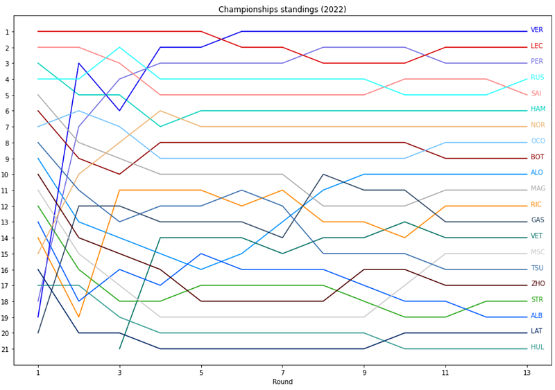
Our second analysis is the overview of the driver standings over time. Which driver is gaining places in the standings and who is loosing places? And when in the season? The graph to realize:

Championship standings (image by author)

First, we need to collect the data to plot this graph. For a given year we need the positions in the drivers world championship after each race.

A method is added to the F1Stats class that returns the WDC (World Driver Championship) standings after each race. A specific year can be selected to filter the data.

The Ergast data set contains a table driver_standings that contains the majority of the required information, but as with the race results some additional data is added about races and drivers. Two consecutive merges add this information (lines 6–10).

For the year 2022 for all rounds (column round) the driver standings are presented in this dataframe. The column position gives the position in the standings and the driver is specified by ID, name and code.

To get the standings after a specific round, the data frame can be filtered on the column ‘round’. To know the position of a specific driver after each round, a filter on his name, code or driverId is possible. When the data contains multiple years, it is the safest to filter on driverId. The driver’s code is definitely not unique over time (e.g. MAG has been used by Jan Magnussen and is in use by Kevin Magnussen), his name might not be.

The method plots for each driver in the dataframe df a line`. It is expected that the dataframe contains a column named ‘code’ with the three letter driver code. For each driver a lines is plotted (lines 6–8), specifying the xcolumn for the x-axis and the ycolumn for the y-axis. In this analysis these are ‘round’ and ‘position’.

The color of the line is driver specific and retrieved from the F1Stats class where a table specifies for each driver the color to represent him on charts. If a driver is not known it returns black.

Lines 9–21 perform some layout functions, like titles, ticks and the axes labels. Lines 22–26 add a label with the driver’s code to the right side of the lines. This all results in:

Driver standings during season 2022 (image by author)

Conclusion

The Ergast data set contains a ton of information on historic Formula 1 races. This article focuses on getting started with this data set, such as importing the data and cleaning the data. Two examples were presented showing a glimpse of the possible analyses to perform.

Take the time to clean up a data set. This helps with the usage of the data and the invested time will be earned back swiftly. When making an analysis, take a step back and think what part of the required data aggregation might be of future use. Add these to the generic class.

More analyses can be found in Analyzing F1 statistics — Part I.

The code for this article can be found in github in the Jupyter notebook named Ergast-analysis.ipynb (including the code for the next article)

Final words

I hope you enjoyed this article. For more inspiration, check some of my other articles:

If you like this story, please hit the Follow button!

Disclaimer: The views and opinions included in this article belong only to the author.