Summary

The article outlines five methods for leveraging histograms to enhance feature engineering in machine learning, including measuring distance between histograms, normalization, altering binning schemes, splitting histograms, and combining them.

Abstract

Histograms play a crucial role in feature engineering for machine learning, offering a way to summarize and visualize data effectively. The article discusses the importance of feature engineering with histograms, emphasizing its impact on the performance of machine learning models. It details five specific techniques: measuring the similarity or dissimilarity of histograms using various distance metrics, normalizing histograms to ensure data is on a comparable scale, adjusting binning schemes to manage dimensionality, splitting histograms to reveal hidden patterns, and combining histograms to create comprehensive features. These methods are presented as tools to make machine learning algorithms more robust and efficient, facilitating better data comparison and model convergence.

Opinions

The author suggests that feature engineering is not just beneficial but essential for the success of machine learning projects.
A variety of distance measures are considered useful for comparing histograms, with the Wasserstein distance highlighted for its versatility in comparing different distributions.
Normalization is advocated for not only improving algorithm performance but also for faster convergence to solutions.
The choice of binning scheme (equal width vs. equal frequency) is presented as a significant decision that can impact the effectiveness of machine learning algorithms.
Splitting histograms is recommended as a technique to make patterns more discernible, aiding in the comparison of multiple datasets.
The article promotes the idea of combining histograms, such as the histogram of oriented gradients with color histograms, to create richer features, potentially enhancing the analysis of complex datasets.

5 Ways to Use Histograms with Machine Learning Algorithms

From a feature engineering perspective

feature engineering with histogram for machine learning (image by author)

Feature engineering is the process of using domain knowledge to create features that make machine learning algorithms work better. This is a crucial part of applied machine learning and is often the difference between successful and unsuccessful projects.

On the other hand, histograms are known as one of the first steps to data preprocessing. It is an essential step for data exploration with simple basics: it summarizes your observations and presents them in a concise way.

But how can we extract features from histograms?

Let’s look at five methods that can help us extract features that can make our models more robust and efficient.

Measure Distance Between Histograms

A distance measure is used to determine how similar or dissimilar two objects are. It is a key element in many machine learning algorithms. A distance function between your feature vectors gives you a way to evaluate whether or not two objects in your dataset are similar.

In other words, it gives you a gauge to evaluate the degree of similarity between two features.

There are many different ways to measure distances, each with its own advantages and disadvantages. The most common distance measures are Euclidean distance, Manhattan distance, and cosine similarity.

But what about the distance between histograms?

Again many methods: the Kullback-Leibler divergence, the chi-squared statistic, exponential divergence, Hellinger distance, the Wasserstein distance…

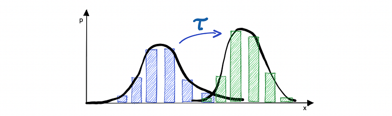
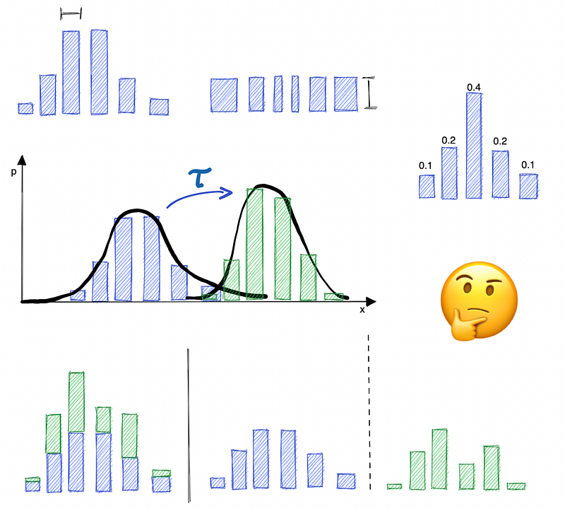
illustration of the distance between two histograms (image by author)

The latter is a very natural metric in the space of probability measures. It is a very versatile metric that measures the amount of “work” needed to change one histogram to another and can be used to compare distributions that are not necessarily identical.

Normalize Histograms

It’s important to normalize data because it can help improve the performance of the algorithms that consume the features. When data is normalized, it means that all the features in the data are on the same scale.

Some algorithms are sensitive to the scale of the data, and normalizing the data can even help some algorithms to converge faster to a solution.

normalized histogram between 0 and 1 (image by author)

But there are also other reasons to normalize histograms:

To make sure that the data is evenly distributed.
To ensure that all data is visible.
To make comparisons between data sets easier.

Change Binning Scheme

For machine learning algorithms that are sensitive to high-dimensional feature vectors, we can reduce the number of dimensions by simply using a smaller number of bins or a smaller range of values.

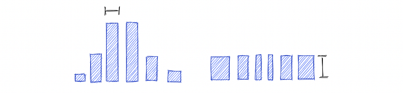
There are two main types of binning schemes:

Equal width binning: In equal width binning, the width of each bin is the same. This is the most common type of binning.
Equal frequency binning: In equal frequency binning, each bin contains the same number of data points.

example of equal width (left) and equal frequency (right) binning (image by author)

There are also other types of binning schemes, but these are the two most common. Equal width binning is the most common type of binning because it is the easiest to implement and straightforward to understand.

Nevertheless, equal frequency binning can be more effective because it ensures that each bin contains the same number of data points.

Split Histograms Into Several Parts

There are several reasons why one might want to split a histogram into several parts. One reason is that it can be easier to compare two or more histograms if they are split into several parts.

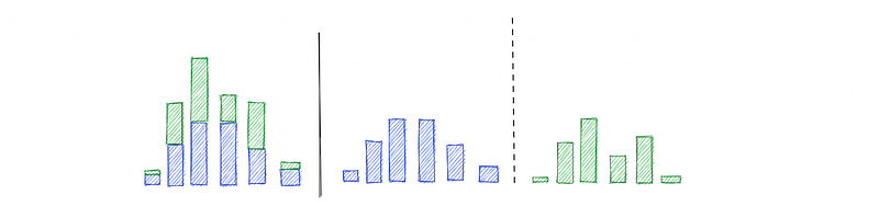
example of a histogram split (image by author)

This is because patterns or trends in the data can become more obvious when split into several parts.

For example, a histogram of the population’s height can be split by geographic area and might reveal that the height distribution is different depending on the country.

Combine histograms

This last part is very specific. Let me explain with an example. Let’s say that we have a dataset of pictures that we want to analyze with the histogram of oriented gradient, but we also want to separate the data depending on their color components.

In that case, we can combine the histogram of oriented gradients with a color histogram as follows.

HOG: [0.01, 0.02, ..]
Color histogram: [0.02, 0.03, ..]
Combined: [0.01, 0.02, .. ,0.02, 0.03, ..]

We can concatenate both histograms and even add weight to each histogram to give more or less importance to one histogram:

Combined with weights: [0.01*w1, 0.02*w1, .. ,0.02*w2, 0.03*w2, ..]

Conclusion

There are a variety of ways to manipulate histograms in order to better understand the data they represent. By measuring the distance between histograms, we can get a sense of how similar or different they are.

We can also normalize histograms to compare them more easily, change the binning scheme to visualize the data better, or split histograms into several parts to better understand the data distribution.

Eventually, we can combine histograms together to form features that can help us solve very specific machine learning problems.

Curious to learn more about Anthony’s work and projects? Follow him on Medium, LinkedIn, and Twitter.

Need a technical writer? Send your request to https://amigocci.io.