3D Python

5-Step Guide to generate 3D meshes from point clouds with Python

Tutorial to generate 3D meshes (.obj, .ply, .stl, .gltf) automatically from 3D point clouds using python. (Bonus) Surface reconstruction to create several Levels of Detail.

In this article, I will give you my 3D surface reconstruction process for quickly creating a mesh from point clouds with python. You will be able to export, visualize and integrate results into your favorite 3D software, without any coding experience. Additionally, I will provide you with a simple way to generate multiple Levels of Details (LoD), useful if you want to create real-time applications (E.g. Virtual Reality with Unity).

3D meshes are geometric data structures most often composed of a bunch of connected triangles that explicitly describe a surface 🤔. They are used in a wide range of applications from geospatial reconstructions to VFX, movies and video games. I often create them when a physical replica is demanded or if I need to integrate environments in game engines, where point cloud support is limited.

They are well integrated in most of the software professionals work with. On top, if you want to explore the wonder of 3D printing, you need to be able to generate a consistent mesh from the data that you have. This article is designed to offer you an efficient workflow in 5 customizable steps along with my script remotely executable at the end of the article. Let us dive in!

Step 1: Setting up the environment

In the previous article, we saw how to set-up an environment easily with Anaconda, and how to use the GUI Spyder for managing your code. We will continue in this fashion, using only 2 libraries.

For getting a 3D mesh automatically out of a point cloud, we will add another library to our environment, Open3D. It is an open-source library that allows the use of a set of efficient data structures and algorithms for 3D data processing. The installation necessitates to click on the ▶️ icon next to your environment.

Open the Terminal and run the following command:

conda install -c open3d-admin open3d==0.8.0.0

🤓 Note: The Open3D package is compatible with python version 2.7, 3.5 and 3.6. If you have another, you can either create a new environment (best) or if you start from the previous article, change the python version in your terminal by typing conda install python=3.5 in the Terminal.

This will install the package and its dependencies automatically, you can just input y when prompted in the terminal to allow this process. You are now set-up for the project.

Step 2: Load and prepare the data

Launch your python scripting tool (Spyder GUI, Jupyter or Google Colab), where we will call 2 libraries: Numpy and Open3D.

import numpy as np
import open3d as o3d

Then, we create variables that hold data paths and the point cloud data:

input_path="your_path_to_file/"
output_path="your_path_to_output_folder/"
dataname="sample.xyz"
point_cloud= np.loadtxt(input_path+dataname,skiprows=1)

🤓 Note: As for the previous post, we will use a sampled point cloud that you can freely download from this repository. If you want to visualize it beforehand without installing anything, you can check the webGL version.

Finally, we transform the point_cloud variable type from Numpy to the Open3D o3d.geometry.PointCloud type for further processing:

pcd = o3d.geometry.PointCloud()
pcd.points = o3d.utility.Vector3dVector(point_cloud[:,:3])
pcd.colors = o3d.utility.Vector3dVector(point_cloud[:,3:6]/255)
pcd.normals = o3d.utility.Vector3dVector(point_cloud[:,6:9])

🤓 Note: The following command first instantiates the Open3d point cloud object, then add points, color and normals to it from the original NumPy array.

For a quick visual of what you loaded, you can execute the following command (does not work in Google Colab):

o3d.visualization.draw_geometries([pcd])

Step 3: Choose a meshing strategy

Now we are ready to start the surface reconstruction process by meshing the pcd point cloud. I will give my favorite way to efficiently obtain results, but before we dive in, some condensed details ar necessary to grasp the underlying processes. I will limit myself to two meshing strategies.

Strategy 1: Ball-Pivoting Algorithm [1]

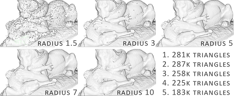
The idea behind the Ball-Pivoting Algorithm (BPA) is to simulate the use of a virtual ball to generate a mesh from a point cloud. We first assume that the given point cloud consists of points sampled from the surface of an object. Points must strictly represent a surface (noise-free), that the reconstructed mesh explicit.

Using this assumption, imagine rolling a tiny ball across the point cloud “surface”. This tiny ball is dependent on the scale of the mesh, and should be slightly larger than the average space between points. When you drop a ball onto the surface of points, the ball will get caught and settle upon three points that will form the seed triangle. From that location, the ball rolls along the triangle edge formed from two points. The ball then settles in a new location: a new triangle is formed from two of the previous vertices and one new triangle is added to the mesh. As we continue rolling and pivoting the ball, new triangles are formed and added to the mesh. The ball continues rolling and rolling until the mesh is fully formed.

The idea behind the Ball-Pivoting Algorithm is simple, but of course, there are many caveats to the procedure as originally expressed here:

• How is the ball radius chosen? The radius, is obtained empirically based on the size and scale of the input point cloud. In theory, the diameter of the ball should be slightly larger than the average distance between points.
• What if the points are too far apart at some locations and the ball falls through? When the ball pivots along an edge, it may miss the appropriate point on the surface and instead hit another point on the object or even exactly its three old points. In this case, we check that the normal of the new triangle Facet is consistently oriented with the point's Vertex normals. If it is not, then we reject that triangle and create a hole.
• What if the surface has a crease or valley, such that the distance between the surface and itself is less than the size of the ball? In this case, the ball would just roll over the crease and ignore the points within the crease. But, this is not ideal behavior as the reconstructed mesh is not accurate to the object.
• What if the surface is spaced into regions of points such that the ball cannot successfully roll between the regions? The virtual ball is dropped onto the surface multiple times at varying locations. This ensures that the ball captures the entire mesh, even when the points are inconsistently spaced out.

Strategy 2: Poisson reconstruction [2]

The Poisson Reconstruction is a bit more technical/mathematical. Its approach is known as an implicit meshing method, which I would describe as trying to “envelop” the data in a smooth cloth. Without going into too many details, we try to fit a watertight surface from the original point set by creating an entirely new point set representing an isosurface linked to the normals. There are several parameters available that affect the result of the meshing:

• Which depth? a tree-depth is used for the reconstruction. The higher the more detailed the mesh (Default: 8). With noisy data you keep vertices in the generated mesh that are outliers but the algorithm doesn’t detect them as such. So a low value (maybe between 5 and 7) provides a smoothing effect, but you will lose detail. The higher the depth-value the higher is the resulting amount of vertices of the generated mesh.

• Which width? This specifies the target width of the finest level of the tree structure, which is called an octree 🤯. Don’t worry, I will cover this and best data structures for 3D in another article as it extends the scope of this one. Anyway, this parameter is ignored if the depth is specified.
• Which scale? It describes the ratio between the diameter of the cube used for reconstruction and the diameter of the samples’ bounding cube. Very abstract, the default parameter usually works well (1.1).

• Which fit? the linear_fit parameter if set to true, let the reconstructor use linear interpolation to estimate the positions of iso-vertices.

Step 4: Process the data

Strategy 1: BPA

We first compute the necessary radius parameter based on the average distances computed from all the distances between points:

distances = pcd.compute_nearest_neighbor_distance()
avg_dist = np.mean(distances)
radius = 3 * avg_dist

In one command line, we can then create a mesh and store it in the bpa_mesh variable:

bpa_mesh = o3d.geometry.TriangleMesh.create_from_point_cloud_ball_pivoting(pcd,o3d.utility.DoubleVector([radius, radius * 2]))

Before exporting the mesh, we can downsample the result to an acceptable number of triangles, for example, 100k triangles:

dec_mesh = mesh.simplify_quadric_decimation(100000)

Additionally, if you think the mesh can present some weird artifacts, you can run the following commands to ensure its consistency:

dec_mesh.remove_degenerate_triangles()
dec_mesh.remove_duplicated_triangles()
dec_mesh.remove_duplicated_vertices()
dec_mesh.remove_non_manifold_edges()

Strategy 2: Poisson’ reconstruction

🤓 Note: The strategy is available starting the version 0.9.0.0 of Open3D, thus, it will only work remotely at the moment. You can execute it through my provided google colab code offered here.

To get results with Poisson, it is very straightforward. You just have to adjust the parameters that you pass to the function as described above:

poisson_mesh = o3d.geometry.TriangleMesh.create_from_point_cloud_poisson(pcd, depth=8, width=0, scale=1.1, linear_fit=False)[0]

🤓 Note: The function output a list composed of an o3d.geometry object followed by a Numpy array. You want to select only the o3d.geometry justifying the [0] at the end.

To get a clean result, it is often necessary to add a cropping step to clean unwanted artifacts highlighted as yellow from the left image below:

For this, we compute the initial bounding-box containing the raw point cloud, and we use it to filter all surfaces from the mesh outside the bounding-box:

bbox = pcd.get_axis_aligned_bounding_box()
p_mesh_crop = poisson_mesh.crop(bbox)

You now have one or more variables that each hold the mesh geometry, well Well done! The final step to get it in your application is to export it!

Step 5: Export and visualize

Exporting the data is straightforward with the write_triangle_mesh function. We just specify within the name of the created file, the extension that we want from .ply, .obj, .stl or .gltf, and the mesh to export. Below, we export both the BPA and Poisson’s reconstructions as .ply files:

o3d.io.write_triangle_mesh(output_path+"bpa_mesh.ply", dec_mesh)
o3d.io.write_triangle_mesh(output_path+"p_mesh_c.ply", p_mesh_crop)

To quickly generate Levels of Details (LoD), let us write your first function. It will be really simple. The function will take as parameters a mesh, a list of LoD (as a target number of triangles), the file format of the resulting files and the path to write the files to. The function (to write in the script) looks like this:

def lod_mesh_export(mesh, lods, extension, path):
    mesh_lods={}
    for i in lods:
        mesh_lod = mesh.simplify_quadric_decimation(i)
        o3d.io.write_triangle_mesh(path+"lod_"+str(i)+extension, mesh_lod)
        mesh_lods[i]=mesh_lod
    print("generation of "+str(i)+" LoD successful")
    return mesh_lods

💡 Hint: I will cover the basics of what the function does and how it is structured in another article. At this point, it is useful to know that the function will (1) export the data to a specified location of your choice in the desire file format, and (2) give the possibility to store the results in a variable if more processing is needed within python.

The function makes some magic, but once executed, it looks like nothing happens. Don’t worry, your program now knows what lod_mesh_export is, and you can directly call it in the console, where we just change the parameters by the desired values:

my_lods = lod_mesh_export(bpa_mesh, [100000,50000,10000,1000,100], ".ply", output_path)

What is very interesting, is that now you don’t need to rewrite a bunch of code every time for different LoDs. You just have to pass different parameters to the function:

my_lods2 = lod_mesh_export(bpa_mesh, [8000,800,300], ".ply", output_path)

If you want to visualize within python a specific LoD, let us say the LoD with 100 triangles, you can access and visualize it through the command:

o3d.visualization.draw_geometries([my_lods[100]])

To visualize outside of python, you can use the software of your choosing (E.g Open-source Blender, MeshLab and CloudCompare) and load exported files within the GUI. Directly on the web through WebGL, you can use Three.js editor or Flyvast to simply access the mesh as well.

Finally, you can import it in any 3D printing software and get quotations about how much it would cost through online printing services 🤑.

Bravo. In this 5-Step guide, we covered how to set-up an automatic python 3D mesh creator from a point cloud. This is a very nice tool that will prove very handy in many 3D automation projects! However, we assumed that the point cloud is already noise-free, and that the normals are well-oriented.

If this is not the case, then some additional steps are needed and some great insights already discussed in the article below will be cover in another article

The full code is accessible here: Google Colab notebook

Conclusion

You just learned how to import, mesh, export and visualize a point cloud composed of millions of points, with different LoD! Well done! But the path does not end here, and future posts will dive deeper in point cloud spatial analysis, file formats, data structures, visualization, animation and meshing. We will especially look into how to manage big point cloud data as defined in the article below.

My contributions aim to condense actionable information so you can start from scratch to build 3D automation systems for your projects. You can get started today by taking a formation at the Geodata Academy

References

1. Bernardini, F.; Mittleman, J.; Rushmeier, H.; Silva, C.; Taubin, G. The ball-pivoting algorithm for surface reconstruction. Transactions on Visualization and Computer Graphics 1999, 5, 349–359.

2. Kazhdan, M.; Bolitho, M.; Hoppe, H. Poisson surface reconstruction. Eurographics symposium on Geometry processing 2006, 1–10.