5 Cool Ways to Enrich ML Models with Open Data for Free: An In-depth Review of Python Libraries

With code examples

Machine learning algorithms are used by numerous businesses to solve a variety of forecasting problems. Predicting the values ​​of time series data is quite common, which has the potential to create business value. For example, a typical task in retail business is to forecast sales in individual stores or in certain categories of goods. Another example is forecasting the demand for rail and air tickets to certain destinations.

All these forecasting problems are strongly tied to the people’s behavior, which is influenced by several factors such as weather, holidays, the state of the economy in the country, and global processes. These factors must be taken into account if you want to build a strong predictive model that produces accurate and robust results.

The number one requirement to create such a model is, of course, data. In this article, we will focus on the task of collecting data and explore 5 popular libraries that gather necessary data for given dates. Moreover, based on the obtained data, we will construct derived features and enrich the training set with them.

We will do an in-depth review of the 5 of the most popular libraries that provide access to different data types:

• 📚holidays — holidays in different countries
• 📚yfinance — stock data from Yahoo Finance
• 📚meteostat — weather data from weather stations around the world
• 📚pandas-datareader — stock data and economic statistics from many sources around the world
• 📚upgini — ready-made features based on many sources

All these libraries can be installed via pip:

pip install holidays yfinance meteostat pandas-datareader upgini

Creating the training data

Let’s imagine we need to solve a very typical problem: Predict the volume of sales for different categories of products in different stores across several countries. We will start with generating a dataset that resembles real sales statistics using Pandas.

1️⃣ The first step is to set a date range, list of countries, stores, and product categories. We will indicate the countries in the form of two-letter ISO codes since most of the aforementioned libraries work exactly with them.

import pandas as pd

start_date = pd.Timestamp("2015-01-01")
end_date = pd.Timestamp("2018-12-31")

countries = ["FI", "SE", "NO"]
stores = ["DataMart", "DataRama"]
products = ["Sticker", "Mug", "Hat"]

2️⃣ The second step is to create a dataset from all combinations of the listed attributes:

index = pd.MultiIndex.from_product(

 [pd.date_range(start_date, end_date), countries, stores, products],
 names=["date", "country", "store", "product"],

)

df = index.to_frame().reset_index(drop=True)

3️⃣ We are ready to generate the sales values. To keep the numbers from being completely random, we will add seasonal and weekly trends, and average sales that vary by country, store, and product. Finally, we will add some random noise. In this step, we will be using functions from the math and random libraries of Python.

from math import pi, sin
from random import random, seed

country_factor = {"FI": 1, "SE": 2, "NO": 3}
store_factor = {"DataMart": 1, "DataRama": 2}
product_factor = {"Sticker": 1, "Mug": 2, "Hat": 3}

seed(0)

def fake_sells(date, country, store, product):
 return int(
    50
    * country_factor[country]
    * store_factor[store]
    * product_factor[product]
    * (1 + 0.25 * sin(2 * pi * date.day_of_year / 365))
    * (1 + 0.1 * sin(2 * pi * date.day_of_week / 7))
    * (1 + 0.4 * random())
  )

df["num_sold"] = df.apply(
   lambda r: fake_sells(
      r["date"], r["country"], r["store"], r["product"]
   ),
   axis="columns",
)

It is important to emphasize that the synthetic data doesn’t contain all the patterns occurring in reality but it will be sufficient to demonstrate the process of enrichment with external features.

✅ We have completed generating the data. Let’s take a look at the first 5 rows of the DataFrame:

df.head()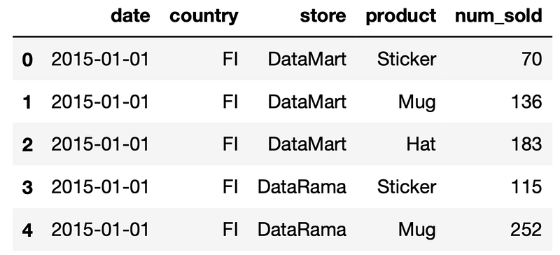

The first library we will cover is the holidays.

📚holidays

It’s natural to expect that holidays have a significant impact on sales. The most popular Python library for getting holiday data is holidays, which allows you to get dates and names of holidays for 86 countries, including those 3 in our dataset.

❗A notable feature of this library is that the holiday schedule is hard coded directly into the library code. On the one hand, this allows you to use it without access to the Internet. However, keep in mind that you will need to update the library each time you want to update information about holidays.

The easiest way to use it is to simply add a column with the names of the holidays for each record. In order not to change the original dataset, we will work with its copy.

🖥️ Demo

import holidays

enriched_df = df.copy()

enriched_df["holiday_name"] = enriched_df.apply(
    
    lambda r: holidays.country_holidays(
        r["country"]).get(r["date"]), 
    axis="columns"
)

Most machine learning libraries can’t use a column with string values ​​directly as a feature. Let’s add a flag for the presence of a holiday for each day:

enriched_df["holiday"] = \
enriched_df["holiday_name"].notna().astype("float")

We will expand the holiday names into one-hot encoded features using the get_dummies function of Pandas:

enriched_df = pd.get_dummies(
    enriched_df, columns=["holiday_name"], prefix="holiday"
)

The features obtained this way contain information on the exact days of the holidays. However, we also observe the effect of a holiday on the sales in the days before and after the holiday.

To construct such features, we need to collect information about holidays not only for the dates presented in the dataset, but also for the dates adjacent to them:

holidays_df = pd.DataFrame(
    [(
        date, 
        country, 
        holidays.country_holidays(country).get(date))
        for country in df["country"].unique()
        for date in pd.date_range(
            start_date - pd.Timedelta(3, "D"), 
            end_date + pd.Timedelta(14, "D")
        )],
    columns=["date", "country", "holiday_name"],
)

We will now transform the names of the holidays into binary features as we have done before:

holidays_df["holiday"] = \
holidays_df["holiday_name"].notna().astype("float")

holidays_df = pd.get_dummies(
    holidays_df, columns=["holiday_name"], prefix="holiday"
)

Let’s construct features that indicate the presence of a particular holiday in the previous 1 or 3 days and in the next 1, 3, 7 or 14 days:

back_features_df = pd.DataFrame(
    {
        f"{column}_d{window_size}_back": (
            holidays_df.groupby("country")[column]
            .rolling(window_size)
            .max()
            .shift(1)
            .values
        )
        for column in holidays_df.columns 
        if column not in ["date", "country"]
        for window_size in [1, 3]
    }
)

ahead_features_df = pd.DataFrame(
    {
        f"{column}_d{window_size}_ahead": (
            holidays_df.groupby("country")[column]
            .rolling(window_size)
            .max()
            .shift(-window_size)
            .values
        )
        for column in holidays_df.columns 
        if column not in ["date", "country"]
        for window_size in [1, 3, 7, 14]
    }
)

holidays_features_df = pd.concat(
    [
        holidays_df[["date", "country"]], 
        back_features_df, 
         ahead_features_df
    ],
    axis=1,
)

We can now enrich our dataset with these features:

enriched_df = enriched_df.merge(
    holidays_features_df, on=["date", "country"]
)

📚yfinance

Shopping behavior is also directly related to the state of the economy and finance in the country and the world. The most accessible and promptly updated indicators of this state are stock indices. To obtain this information, we will use the yfinance library.

To get the data, we need to define a set of indices and a time interval. For demonstration purposes, we will get only the main American and European stock indices (S&P500, NASDAQ, Dow Jones, STOXX), commodity prices (gold, silver, oil, gas) and currencies (dollar index, euro/dollar exchange rate).

🖥️ Demo

tickers = {
    "^GSPC": "snp500",
    "^IXIC": "nasdaq",
    "^DJI": "dow_jones",
    "^STOXX": "stoxx",
    "GC=F": "gold",
    "SI=F": "silver",
    "CL=F": "crude_oil",
    "NG=F": "natural_gas",
    "DX-Y.NYB": "usd",
    "EUR=X": "eur",
}

The next step is to build features by aggregating data over large windows. Let’s download the data for the time period extended accordingly:

import yfinance as yf

start_date = pd.Timestamp("2015-01-01")
end_date = pd.Timestamp("2018-12-31")
forecast_shift = pd.Timedelta(7, "D")

yfinance_df = yf.download(
    list(tickers),
    start=start_date - forecast_shift - pd.Timedelta(365 + 7, "D"),
    end=end_date,
)

Unlike holidays, stock prices data is not known in advance. We will predict the sales for a week ahead which is the reason why we have added a forecast shift of 7 days. We must fit the model on features from the forecast date minus 7 days.

Several indicators are available for each trading day, such as the opening price or trading volume. We will keep only the adjusted closing price. Let’s also rename the columns for better readability:

yfinance_df = yfinance_df["Adj Close"]
yfinance_df = yfinance_df.rename(columns=tickers)
yfinance_df.index.name = "date"

There is no stock data for non-working days. Let’s fill them with the previous available values:

yfinance_df = yfinance_df.fillna(method="ffill")
yfinance_df = yfinance_df.asfreq("D", method="ffill")

Only data known in advance can be used to build forecasts for the future. Let’s shift the dates to our forecasting horizon:

yfinance_df.index += forecast_shift

In addition to the raw values, let’s also create some derivatives:

• The ratio of the current value to the average for the past 7 days
• The ratio of the average for 7 days to the average for the year
• The ratio of the average for 7 days to the same period of the last year

yfinance_features_df = pd.concat(
    [
        yfinance_df,
        (
            yfinance_df / yfinance_df.rolling(7).mean()
        ).add_suffix("_1d_to_7d"),
        (
            yfinance_df.rolling(7).mean() / 
            yfinance_df.rolling(365).mean()
        ).add_suffix("_7d_to_1y"),
        (
            yfinance_df.rolling(7).mean() /  
            yfinance_df.shift(365).rolling(7).mean()
        ).add_suffix("_7d_to_7d_1y_shift"),
    ],
    axis=1,
).dropna()

Finally, we will enrich the original dataset with these features:

enriched_df = df.merge(yfinance_features_df, on="date")

The enriched dataset has 45 features. You can view them using the head method or columns method of DataFrame.

📚meteostat

The weather conditions certainly affect the sales of commodities in many categories, from soft drinks to heating devices. The meteostat library allows you to get historical data from many weather stations around the world.

Among the available indicators are the average, maximum and minimum temperature per day, atmospheric pressure, the amount of precipitation and wind speed.

Since we don’t have exact coordinates of stores, we’ll take the average values for each country. For these purposes, the library provides the ability to request a list of all weather stations in the country, as well as an easy-to-use method for aggregating their readings.

To obtain more stable features, we will keep only stations that have a continuous history of daily observations during the time period we are interested in.

🖥️ Demo

from meteostat import Daily, Stations
 
meteostat_dfs = []
 
for country in df["country"].unique():
    stations = Stations().region(country).fetch()
    stations = stations[
        (stations["daily_start"] <= start_date - forecast_shift)
        & (stations["daily_end"] >= end_date)
    ]
    meteostat_df = (
        Daily(stations, start_date - forecast_shift, end_date)
        .normalize()
        .aggregate(spatial=True)
        .fetch()
    )
    meteostat_df.index.name = "date"
    meteostat_df["country"] = country
    meteostat_dfs.append(meteostat_df)
 
meteostat_features_df = pd.concat(meteostat_dfs)

❗Unfortunately, the library incorrectly calculates the average of wind direction when aggregating over several stations. In addition, some of the columns may contain a lot of missing values. Let’s keep only well-filled columns:

meteostat_features_df = meteostat_features_df[
    [
        "country", 
        "tavg", 
        "tmin", 
        "tmax", 
        "prcp", 
        "snow", 
        "wspd", 
        "pres"
    ]
]

We will add a date shift for our forecasting horizon:

meteostat_features_df.index += forecast_shift

Finally, we can enrich the original dataset with weather features:

enriched_df = df.merge(
    meteostat_features_df, 
    on=["date", "country"]
)

📚pandas-datareader

Pandas-datareader provides an interface for accessing a large number of data sources. Currently, 16 active sources are supported. 11 of them contain mainly stock and financial data and the remaining 5 contain various economic statistics.

❗Some sources limit the amount of data available for free. You must be ready for registration and obtaining personal keys.

We have already used the yfinance library for stock prices data. Thus, we turn to economic statistics and get the Consumer Price Index (CPI). It indicates the level of prices for different categories of consumer goods and services, which directly affects the people’s purchasing power.

CPI values ​​are updated monthly. In addition to the raw value of this indicator, the change relative to the previous month or the corresponding month of the previous year are also available.

❗CPI can be obtained from several sources but it’s not very easy. We first have to look for it on each site. This is the downside of using the pandas-datareader library: it doesn’t provide a single searchable catalog of available datasets. In this case, it turned out that EconDB would be a convenient source for CPI.

Let’s construct in the request by placing the name of the dataset (IMF_CPI), the country filter, the data frequency (M — monthly), and the date range. We should take into account that data for any month becomes available only in the month following after. Therefore, we will extend the range for an additional 1 month.

🖥️ Demo

import pandas_datareader.data as web
 
datareader_df = web.DataReader(
    "&".join(
        [
            "dataset=IMF_CPI",
            f"REF_AREA=[{','.join(countries)}]",
            "FREQ=[M]",
            f"from={start_date - forecast_shift -  
               pd.DateOffset(months=1, day=1):%Y-%m-%d}",
            f"to={end_date:%Y-%m-%d}",
        ]
    ),
    "econdb",
)

The downloaded dataset contains only entries for the first day of each month. To be able to join it on any date, we will fill in the rest of the dates of the month with the same value. We will also shift the dates according to the data availability at the time of the forecast:

datareader_df.index += pd.DateOffset(months=1)
datareader_df = datareader_df.asfreq("D", method="ffill")
datareader_df.index += forecast_shift

Let’s move countries from the columns to the rows using the stack method and rename the columns:

datareader_features_df = datareader_df.stack("Reference Area")
datareader_features_df = datareader_features_df.droplevel(
   ["Frequency", "Scale"], axis="columns"
)

datareader_features_df = datareader_features_df.rename_axis(
   ("date", "country")
)

Finally, let’s replace the country names with ISO codes:

country_codes = {"Finland": "FI", "Sweden": "SE", "Norway": "NO"}
datareader_features_df = datareader_features_df.reset_index()

datareader_features_df["country"] = \
datareader_features_df["country"].replace(
    country_codes
)

We can now enrich the original dataset:

enriched_df = df.merge(
    datareader_features_df, 
    on=["date", "country"]
)

The enriched dataset has 131 features. You can view them using the head method or columns method of DataFrame.

❗Here is a list of things you should keep in mind before starting to work with pandas-datareader:

• The data loading speed is highly dependent on the source and varies from seconds to minutes. It is sometimes interrupted due to a timeout.
• You need to deal with each data source separately: what attributes are available, whether registration is required, query syntax, etc.
• No guarantees: the library is a connector and is not responsible for the availability of data.
• It’s impossible to get different data for comparison and evaluation with one request. You need to query each indicator separately.

📚upgini

Upgini aggregates a lot of open data sources with a wide range of keys and their combinations (dates, countries, postal codes, IP addresses, phone numbers, emails). In this review, we will focus only on date and country. For these keys, Upgini provides access to all the data types discussed above, as well as the schedule of major international and national events such as olympiads and elections.

The main differences between using Upgini and collecting features from separate sources on your own are:

• All sources are requested simultaneously with a single request.
• Joining by keys occurs automatically.
• The result of enrichment is not raw data, but normalized, cleaned up and transformed features, ready for use in any model.
• The service returns only those features that contain useful information for the specified target prediction.

Thanks to these advantages, using Upgini comes down just to the following few lines.

🖥️ Demo

from upgini import FeaturesEnricher, SearchKey

X = df.drop(columns="num_sold")
y = df["num_sold"]

enricher = FeaturesEnricher(
    search_keys={
        "date": SearchKey.DATE,
        "country": SearchKey.COUNTRY,
    }
)

enriched_df = enricher.fit_transform(X, y, keep_input=True)

As a result, we get the original dataset enriched with more than a hundred of features from different sources. Each returned feature passes a selection stage. The selection criterion applied is the contribution of a feature to the prediction of the target variable that we specified in a fit call. Additionally, SHAP values for each feature are returned and can be used for further independent selection of features.

As an outcome, with a single request, Upgini performs many steps of a standard ML pipeline at once: data extraction, data cleaning, feature engineering, and feature selection.

Comparison and conclusions

holidays

😊 Pros

• Works without an internet access
• Quick responses

👎 Cons

• The holiday schedule in the past is often incorrect
• No information about ad hoc holiday transfers
• No information on other non-working days, including one-time events such as COVID lockdowns
• No holiday categorization or matching of holiday names in different languages
• No information about holidays that are working days
• Limited countries coverage

💥 Usage recommendations

Before using this library, make sure that the countries you are interested in are included in the list of supported ones. If you need information about the full working / weekend schedule, then you’ll have to add the necessary information yourself.

The library can be used if you need only the information about the dates and names of holidays and the requirements for the completeness and accuracy of the data are not very high. If you need consistent historical information on holiday schedules and holiday transfers, as an example, for training of machine learning algorithms, then it’s better to use other tools to get it.

yfinance

😊 Pros

• Quick responses
• Intraday data
• Access to most of the world’s exchanges
• Data for almost 100 years

👎 Cons

• Prohibition on the using of Yahoo Finance data for commercial purposes
• No API access guarantee
• Intraday data is only available for the last 60 days
• Impossible to get full list of available tickers
• Impossible to download all the instruments from a certain exchange or a certain index without a complete enumerating all of them

💥 Usage recommendations

The library can be used for research or educational purposes only. If you are engaged in trading strategies or other tasks related to finance, this type of data will be useful for your purposes. But in any case, you’ll have to transform raw data into features suitable for use in machine learning models.

meteostat

😊 Pros

• No restrictions on the use of data, including commercial purposes (except for the distribution of the original data without modifications)
• Global coverage
• Over 200 hundred years of data history
• Local caching to disk to optimize repeated requests

👎 Cons

• Even if you specify a short time interval, the history of observations for the weather station is downloaded entirely, which affects the speed of requests
• Weather stations are unevenly distributed and the accuracy of data for given coordinates will vary greatly in different parts of the world
• Lots of missing data, part of the gaps replaced by simulated data
• Calculation of the average wind direction when averaging data from several weather stations is implemented incorrectly

💥 Usage recommendations

The library provides maximum data coverage both geographically and chronologically, but the quality suffers due to the large number of gaps in the data. Be careful when choosing the nearest weather station to the coordinates you need. Probably it’s better to choose a more distant weather station, but with better data completeness.

There are no weather forecasts in meteostat and the data is updated with a delay, so if you need the most recent data or forecasts for the next dates, then you should look for another data source.

pandas-datareader

😊 Pros

• Wide range of sources including data aggregators
• Access to high-quality commercial stock data sources

👎 Cons

• No unified API for accessing different sources. To make certain queries you’ll have to study the source sites
• No guarantee that the source will work
• Different licensing restrictions on the use of data for different sources, up to paid access for some of them
• Impossible to get a list of available data either for individual sources or for all sources at once (you need to study the source sites yourself)
• Many data columns are duplicated in different sources, but with different completeness, updating frequency, and depth of available history
• Impossible to request multiple datasets with a single query
• Download speed varies greatly between sources, up to the inability to get some data due to timeouts

💥 Usage recommendations

This library provides the widest coverage of financial, economic, demographic statistics at country level. This kind of data can be very useful for building long-term economic models. But to solve typical business problems, country level granularity and monthly/annual frequency of measurements will not be enough. If you need to plan the supply of goods to different stores for the next two weeks, then instead of global macroeconomic trends, it’s better to look for more localized and frequent data.

You should also take into account the difficulty in finding relevant data. If you don’t know exactly what kind of information you need, then pandas-datareader probably won’t work for you.

upgini

😊 Pros

• Wide variety of data types
• Localization of data down to a country level or postal code where possible
• A lot of extra data keys for enrichment — “country”, “zip code”, “phone number”, “hashed email”, “IP address”
• Ready-made features for ML models
• Simple Scikit-Learn compatible API to get all the data with a single request
• Automatic selection of relevant features for the target variable
• SHAP values for collected features to facilitate further selection steps
• Convenient enrichment of new data batches with the saved search result

👎 Cons

• Relatively low response time (several minutes)
• You can’t choose the types of requested data or specific features yourself, all of them are automatically selected and ranked
• Features are always selected for a specific target variable, so the enrichment results can’t be reused for another task
• There’s no detailed description of the features, which makes the interpretation difficult for some of them

💥 Usage recommendations

If your goal is to train machine learning models, then this library is just perfect, thanks to ready-made relevant features and transparent integration into Scikit-Learn.

You can become a Medium member to unlock full access to my writing, plus the rest of Medium. If you already are, don’t forget to subscribe if you’d like to get an email whenever I publish a new article.

Thank you for reading. Please let me know if you have any feedback.