
5 Convenient File Formats to Save the Preprocessed Data for Machine Learning
It is essential to save the prepared datasets for future use or sharing with others
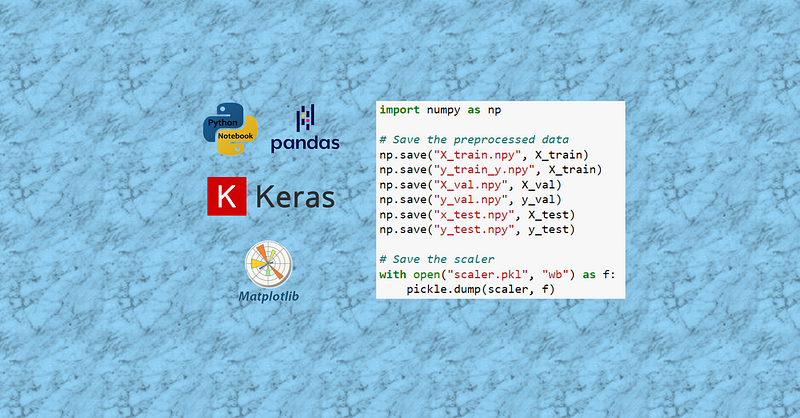
Table of Contents:
∘ Introduction: ∘ 1. Load a Dataset ∘ 2. Prepare the dataset: ∘ 3. Save the prepared data ∘ (1) Save as Pandas DataFrame ∘ (2) Save as NumPy arrays: ∘ (3) Save as HDF5 file: ∘ (4) Save as TensorFlow Datasets: ∘ (5) Save as a pickle file ∘ 4. Load the saved date back ∘ (1) Load the CSV files: ∘ (2) Loading from NumPy arrays: ∘ (3) Loading from HDF5 files: ∘ (4) Loading from TensorFlow Datasets: ∘ (5) Loading from pickle files: ∘ 5. Advantages and disadvantages of the different file formats ∘ (1) CSV Files: ∘ (2) NumPy Arrays: ∘ (3) HDF5 Files: ∘ (4) TensorFlow Datasets: ∘ (5) Pickle Files: ∘ Conclusion:
Introduction:
When working with prepared datasets, it is essential to save them for future use or sharing with others. There are various methods available to save prepared data, including input sequences, output sequences, validation and test sets, and any accompanying objects like scalers. Each method offers its advantages and considerations, depending on the nature of the data and the intended use. In this response, we will explore practical methods such as saving as CSV files, NumPy arrays, HDF5 files, and using pickle files. Let’s now summarize the discussed methods and conclude their benefits using the dataset of ‘apple_share_price.csv’.
1. Load a Dataset
You can start by loading the dataset from the provided URL using libraries like pandas or numpy. Here’s an example:
import pandas as pd

url = "https://raw.githubusercontent.com/shoukewei/data/main/data-wpt/USD_CNY%20Historical%20Data.csv"
data = pd.read_csv(url)
data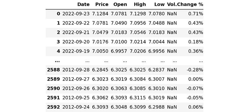
# Sort the dataset by date
df = data.sort_values('Date').reset_index(drop=True)

# Convert the 'Date' column to datetime
df['Date'] = pd.to_datetime(df['Date'])
df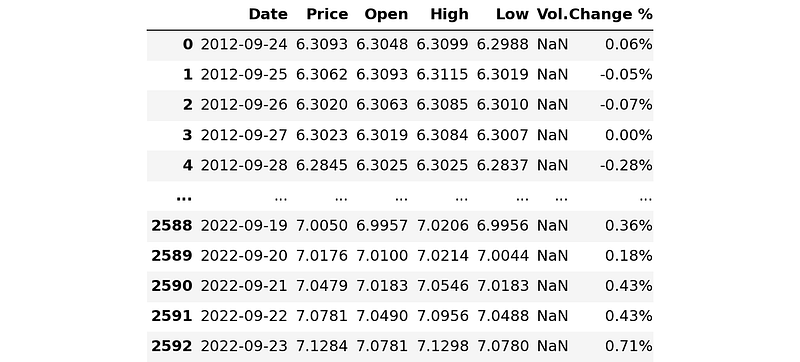
2. Prepare the dataset:
Once you have loaded the dataset, you need to preprocess it according to your requirements. This may involve cleaning the data, feature engineering, splitting into input and output sequences, and normalizing the data using a scaler. Here’s an example:
from sklearn.preprocessing import MinMaxScaler
from sklearn.model_selection import train_test_split

# Extract the "Close" prices
prices = df["Price"].values.reshape(-1, 1)

# Scale the data
scaler = MinMaxScaler()
scaled_prices = scaler.fit_transform(prices)

# Function to create input and output sequences
def create_sequences(data, seq_length):
    X = []
    y = []
    for i in range(len(data) - seq_length):
        sequence = data[i : i + seq_length]
        target = data[i + seq_length]
        X.append(sequence)
        y.append(target)
    return np.array(X), np.array(y)

# Define the sequence length
sequence_length = 10  # Adjust as needed

# Create input and output sequences
X, y = create_sequences(scaled_prices, sequence_length)

# Split into train, validation, and test sets
X_train, X_test, y_train, y_test = train_test_split(X, y, test_size=0.2, shuffle=False)
X_train, X_val, y_train, y_val = train_test_split(X_train, y_train, test_size=0.15, shuffle=False)

# Print the shapes of the datasets
print("Train X shape:", X_train.shape)
print("Train y shape:", y_train.shape)
print("Validation X shape:", X_val.shape)
print("Validation y shape:", y_val.shape)
print("Test X shape:", X_test.shape)
print("Test y shape:", y_test.shape)
In the above code, we first scale the selected date with MinMaxScaler function of scikit-learn, and define a function of create_sequences to create input and output sequences. The create_sequences function takes the data and sequence length as inputs and returns the input sequences X and output sequences y. It uses a sliding window approach to create the sequences. The scikit-learn's train_test_split function is then used to split the data into train, validation, and test sets based on the specified test and validation sizes.
3. Save the prepared data
To save the prepared dataset, you can use various methods. In this section, we will see some essential methods as follows.
(1) Save as Pandas DataFrame
The first method that we usually use is to save the prepared data as Pandas DataFrame.
import pandas as pd
import numpy as np

# Reshape the arrays to 2-dimensional
X_train_2d = X_train.reshape(X_train.shape[0], -1)
y_train_2d = y_train.reshape(y_train.shape[0], -1)
X_val_2d = X_val.reshape(X_val.shape[0], -1)
y_val_2d = y_val.reshape(y_val.shape[0], -1)
X_test_2d = X_test.reshape(X_test.shape[0], -1)
y_test_2d = y_test.reshape(y_test.shape[0], -1)

# Save the preprocessed data as CSV files
pd.DataFrame(X_train_2d).to_csv("X_train.csv", index=False)
pd.DataFrame(y_train_2d).to_csv("y_train.csv", index=False)
pd.DataFrame(X_val_2d).to_csv("X_val.csv", index=False)
pd.DataFrame(y_val_2d).to_csv("y_val.csv", index=False)
pd.DataFrame(X_test_2d).to_csv("X_test.csv", index=False)
pd.DataFrame(y_test_2d).to_csv("y_test.csv", index=False)
The arrays ‘X_train’, ‘y_train’, ’X_val’, ‘y_val’, ‘X_testn’, and ‘y_test’ are reshaped using the reshape method to convert them into 2-dimensional arrays. The '-1' argument in the reshape ensures that the shape is adjusted based on the original dimensions. Then, the reshaped arrays are saved as CSV files using the 'to_csv' method.
(2) Save as NumPy arrays:
Instead of saving the dataset as CSV files, you can save them as NumPy arrays using the numpy.save() function. Here's an example:
import numpy as np

# Save the preprocessed data
np.save("X_train.npy", X_train)
np.save("y_train_y.npy", X_train)
np.save("X_val.npy", X_val)
np.save("y_val.npy", y_val)
np.save("x_test.npy", X_test)
np.save("y_test.npy", y_test)

# Save the scaler
with open("scaler.pkl", "wb") as f:
    pickle.dump(scaler, f)
This method saves the arrays in a binary format, which is more efficient for large datasets.
(3) Save as HDF5 file:
HDF5 (hierarchical data format) is a popular file format for storing large numerical datasets. You can use the ‘h5py’ library to save the prepared dataset as an HDF5 file. Here’s an example:
import h5py

# Save the preprocessed data
with h5py.File("dataset.h5", "w") as f:
    f.create_dataset("X_train", data=X_train)
    f.create_dataset("y_train", data=y_train)
    f.create_dataset("X_val", data=X_val)
    f.create_dataset("y_val", data=y_val)
    f.create_dataset("X_test", data=X_test)
    f.create_dataset("y_test", data=y_test)

# Save the scaler
with open("scaler.pkl", "wb") as f:
    pickle.dump(scaler, f)
This method allows you to store multiple datasets in a single file with a hierarchical
(4) Save as TensorFlow Datasets:
If you’re working with TensorFlow, you can save the prepared dataset as a TensorFlow Dataset using the tf.data.Dataset.save() function. Here’s an example:
import tensorflow as tf
import pickle

# Convert arrays to TensorFlow Datasets
train_dataset = tf.data.Dataset.from_tensor_slices((X_train, y_train))
validation_dataset = tf.data.Dataset.from_tensor_slices((X_val, y_val))
test_dataset = tf.data.Dataset.from_tensor_slices((X_test, y_test))

# Save the datasets
tf.data.Dataset.save(train_dataset, "train_dataset")
tf.data.Dataset.save(validation_dataset, "validation_dataset")
tf.data.Dataset.save(test_dataset, "test_dataset")

# Save the scaler
with open("scaler.pkl", "wb") as f:
    pickle.dump(scaler, f)
This method is useful if you want to leverage the TensorFlow ecosystem for data loading and processing.
(5) Save as a pickle file
Pickle can easily save the prepared dataset as a dictionary. Here is an example:
import pickle

# Save the preprocessed data
with open("dataset.pkl", "wb") as f:
    pickle.dump({
        "X_train": X_train,
        "y_train": y_train,
        "X_val": X_val,
        "y_val": y_val,
        "X_test": X_test,
        "y_test": y_test
    }, f)

# Save the scaler
with open("scaler.pkl", "wb") as f:
    pickle.dump(scaler, f)
In this example, the prepared dataset is saved as a dictionary containing the different data splits. The dictionary is then dumped into a pickle file named “dataset.pkl”. The scaler is saved separately in the “scaler.pkl” file.
4. Load the saved date back
When we use the prepare date for a machine learning, we can easily load them back. Let’s go through the examples.
(1) Load the CSV files:
import pandas as pd

# Load X_train and y_train
X_train = pd.read_csv('X_train.csv')
y_train = pd.read_csv('y_train.csv')

# Load X_val and y_val
X_val = pd.read_csv('X_val.csv')
y_val = pd.read_csv('y_val.csv')

# Load X_test and y_test
X_test = pd.read_csv('X_test.csv')
y_test = pd.read_csv('y_test.csv')
(2) Loading from NumPy arrays:
import numpy as np

# Load X_train and y_train
X_train = np.load('X_train.npy')
y_train = np.load('y_train.npy')

# Load X_val and y_val
X_val = np.load('X_val.npy')
y_val = np.load('y_val.npy')

# Load X_test and y_test
X_test = np.load('X_test.npy')
y_test = np.load('y_test.npy')
(3) Loading from HDF5 files:
import h5py

# Load the HDF5 file
with h5py.File('dataset.h5', 'r') as f:
    # Load datasets from the file
    X_train = f['X_train'][:]
    y_train = f['y_train'][:]
    X_val = f['X_val'][:]
    y_val = f['y_val'][:]
    X_test = f['X_test'][:]
    y_test = f['y_test'][:]
(4) Loading from TensorFlow Datasets:
import tensorflow as tf
import pickle

# Load the TensorFlow Datasets
train_dataset = tf.data.experimental.load("train_dataset", element_spec=(tf.TensorSpec(shape=(), dtype=tf.string),
                                                                         tf.TensorSpec(shape=(), dtype=tf.float32)))
validation_dataset = tf.data.experimental.load("validation_dataset", element_spec=(tf.TensorSpec(shape=(), dtype=tf.string),
                                                                                   tf.TensorSpec(shape=(), dtype=tf.float32)))
test_dataset = tf.data.experimental.load("test_dataset", element_spec=(tf.TensorSpec(shape=(), dtype=tf.string),
                                                                       tf.TensorSpec(shape=(), dtype=tf.float32)))

# Load the scaler object
with open("scaler.pkl", "rb") as f:
    scaler = pickle.load(f)
(5) Loading from pickle files:
import pickle

# Load the preprocessed data
with open("dataset.pkl", "rb") as f:
    data = pickle.load(f)

X_train = data["X_train"]
y_train = data["y_train"]
X_val = data["X_val"]
y_val = data["y_val"]
X_test = data["X_test"]
y_test = data["y_test"]

# Load the scaler object
with open("scaler.pkl", "rb") as f:
    scaler = pickle.load(f)
5. Advantages and disadvantages of the different file formats
(1) CSV Files:
Advantages:
Easy to understand and widely supported by various tools and platforms. Human-readable format, which facilitates data inspection and manual modifications. Can handle tabular data with different data types.
Disadvantages:
Can be less efficient for large datasets due to the text-based nature of the format. May require additional parsing and data type conversions when reading the data.
(2) NumPy Arrays:
Advantages:
Efficient storage and retrieval of numerical data. Seamless integration with scientific computing libraries like NumPy and Pandas. Preserves the original data type and dimensions.
Disadvantages:
Requires additional code to save and load the arrays compared to CSV files. Not human-readable, making it harder to inspect or modify the data manually.
(3) HDF5 Files:
Advantages:
Supports high-performance I/O operations for large datasets. Can store multiple datasets and complex hierarchical structures within a single file. Efficient compression capabilities to reduce storage size. Compatible with various programming languages.
Disadvantages:
Requires additional libraries (e.g., h5py, PyTables) to work with the data. Not as widely supported by all tools and platforms compared to CSV files.
(4) TensorFlow Datasets:
Advantages:
Specifically designed for TensorFlow, providing seamless integration with TensorFlow workflows. Offers built-in functionality for data loading, preprocessing, and batching. Can be easily shared and reused within the TensorFlow ecosystem.
Disadvantages:
Limited compatibility with non-TensorFlow frameworks or tools. May require additional code or conversion steps to work with other machine learning libraries.
(5) Pickle Files:
Advantages:
Supports serialization of complex data structures and objects. Preserves the internal structure and relationships of the data. Can store arbitrary Python objects along with the data.
Disadvantages:
Not human-readable, making it harder to inspect or modify the data manually. Requires the same version of Python and associated libraries for loading the pickle files. Consider these advantages and disadvantages when choosing the appropriate file format for your specific use case. Factors such as data size, compatibility requirements, ease of use, and integration with your preferred tools should influence your decision.
Conclusion:
Saving prepared datasets is crucial for reproducibility and sharing with others. We explored several practical methods for saving prepared data, including input sequences, output sequences, validation and test sets, and associated objects like scalers. The methods discussed were:
- Saving as CSV files: This method allows for easy data storage and compatibility with various tools, but it may be less efficient for large datasets.
- Saving as NumPy arrays: Saving datasets as NumPy arrays offers efficient storage and easy integration with other scientific computing libraries.
- Saving as HDF5 files: HDF5 files are suitable for handling large datasets and provide a hierarchical structure for organizing data.
- Saving as TensorFlow Datasets: This method is advantageous when working with TensorFlow and leverages its data loading and processing capabilities.
- Saving as pickle files: Pickle files enable the storage of complex data structures and trained objects, making them convenient for preserving datasets and associated objects in a serialized format.
Each method has its strengths and considerations, such as file size, compatibility, and integration with specific libraries. Consider the requirements of your project, the nature of the data, and the tools you are using to choose the most suitable method for saving your prepared dataset.


