
Data Science
5 Advanced SQL Concepts You Should Know in 2022
Master these time-saving, advanced SQL queries today

Be a pro in SQL! 🏆
SQL or Structured Query Language is a must have tool for anyone who works with data.
With the rising volume of data, the need for skilled data professionals is also increasing. Only knowledge of advanced SQL concepts is not enough, but you should be able to implement them at your work efficiently And that is what looked for in job interviews for data science positions!
Therefore, I listed here 5 advanced SQL concepts with explanations and query examples which you should know in 2022.
I kept this article pretty short, so that you can finish it quickly and master the must-know, interview-winning SQL tricks. 🏆
You can quickly navigate to your favorite part using this index.
· Common Table Expressions (CTEs)
· ROW_NUMBER() vs RANK() vs DENSE_RANK()
· CASE WHEN Statement
· Extract Data From Date — Time Columns
· SELF JOIN
📍 Note: I’m using SQLite DB Browser and a self created Dummy_Sales_Data created using Faker which you can get on my Github repo for Free!
Okay, here we go…🚀
Common Table Expressions (CTEs)
While working with real world data, sometimes you need to query the results of another query. A simple way to achieve this is to use sub-query.
However, with increasing complexity, computations sub-queries become difficult to read and debug.
That’s when the CTEs come into picture to make your life easier. CTEs make it easy to write and maintain complex queries. ✅
for example, consider the following data extraction using sub-query
SELECT Sales_Manager, Product_Category, UnitPrice
FROM Dummy_Sales_Data_v1
WHERE Sales_Manager IN (SELECT DISTINCT Sales_Manager
                        FROM Dummy_Sales_Data_v1
                        WHERE Shipping_Address = 'Germany'
                        AND UnitPrice > 150)
AND Product_Category IN (SELECT DISTINCT Product_Category
                         FROM Dummy_Sales_Data_v1
                         WHERE Product_Category = 'Healthcare'
                         AND UnitPrice > 150)
ORDER BY UnitPrice DESC
Here I used only two sub-queries with easy to understand code.
It is still difficult to follow, what about when you add more calculations within sub-queries or even add few more sub-queries — complexity increases making the code less readable and difficult to maintain.
Now, let’s see the simplified version of above sub-query with CTE as below.
WITH SM AS
(
SELECT DISTINCT Sales_Manager
FROM Dummy_Sales_Data_v1
WHERE Shipping_Address = 'Germany'
AND UnitPrice > 150
),
PC AS
(
SELECT DISTINCT Product_Category
FROM Dummy_Sales_Data_v1
WHERE Product_Category = 'Healthcare'
AND UnitPrice > 150
)SELECT Sales_Manager, Product_Category, UnitPrice
FROM Dummy_Sales_Data_v1
WHERE Product_Category IN (SELECT Product_Category FROM PC)
AND Sales_Manager IN (SELECT Sales_Manager FROM SM)
ORDER BY UnitPrice DESCThe complex sub-query is decomposed into simpler block of codes to be used.
In this way, the complex sub-queries are re-written into two CTEs SM and PC which are easier to understand and modify. 🎯
Both the above queries, taking same time to execute resulted into the same output as below.
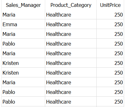
CTEs essentially allow you to create a temporary table from the result of a query. This improves code readability and its maintenance. ✅
The real world data sets can have millions or billions rows occupying 1000s of GB storage. Making calculations using data from these tables and especially joining them with other tables directly will be quite expensive.
An ultimate solution for such tasks is to use CTEs. 💯
Going ahead, let’s see how you can assign an integer ‘rank’ to each row in the data set using window functions.
ROW_NUMBER() vs RANK() vs DENSE_RANK()
Another commonly used concept while working with real data sets is ranking of records. Companies use it in different scenarios such as —
- Ranking top selling brands by number of units sold
- Ranking top product verticals by number of orders or revenue generated
- Getting movie name in each genres with highest number of views
ROW_NUMBER , RANK() and DENSE_RANK() are essentially used to assign sequential integers to each record within mentioned partition of the result set.
Difference between them is visible when you have ties on certain records.
The behavior and the way in which integers are assigned to each record changes when there are duplicate rows in resulting table. ✅
Let’s have a quick example of Dummy Sales Dataset to list all the product categories, shipping address by descending order of shipping cost.
SELECT Product_Category,
  Shipping_Address,
  Shipping_Cost,
  ROW_NUMBER() OVER
              (PARTITION BY Product_Category,
                            Shipping_Address
               ORDER BY Shipping_Cost DESC) as RowNumber,
  RANK() OVER
        (PARTITION BY Product_Category,
                      Shipping_Address
         ORDER BY Shipping_Cost DESC) as RankValues,
  DENSE_RANK() OVER
              (PARTITION BY Product_Category,
                            Shipping_Address
               ORDER BY Shipping_Cost DESC) as DenseRankValues
FROM Dummy_Sales_Data_v1
WHERE Product_Category IS NOT NULL
AND Shipping_Address IN ('Germany','India')
AND Status IN ('Delivered')
As you can see, the syntax for all the three is same, however, it results in different outputs as below,
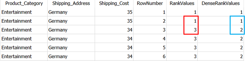
RANK() is retrieves ranked rows based on the condition of ORDER BY clause. As you can see there is a tie between 1st two rows i.e. first two rows have same value in Shipping_Cost column (which is mentioned in ORDER BY clause).
RANK assigns the same integer to both the rows. However, it adds the number of repeated rows to the repeated rank to get the rank of the next row. That’s why, the third row (marked in Red), RANK assigns the rank 3 (2 repeated rows + 1 repeated rank)
DENSE_RANK is similar to the RANK, but it does not skip any numbers even if there is a tie between the rows. This you can see in Blue box in the above picture.
Unlike above two, ROW_NUMBER simply assigns sequential numbers to each record in partition starting with 1. If it detects two identical values in the same partition, it assigns different rank numbers to both.
For the next partition of product category — shipping address → Entertainment — India, the ranks by all three functions re-start with 1, as shown below.
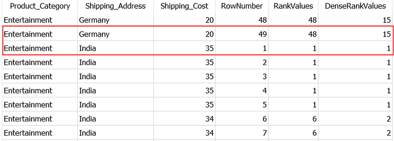
Ultimately, if there are no duplicated values in the column used in the ORDER BY clause, these functions will return the same output. 💯
Going ahead, next concept will tell more about how to implement conditional statements and pivot data using that.
CASE WHEN Statement
CASE statement will allow you to implement if-else in SQL, so you can use it to run the query conditionally.
CASE statement will essentially tests conditions mentioned in WHEN clause and returns the value mentioned in THEN clause. When no condition is satisfied, it will return the value mentioned in the ELSE clause. ✅
While working on the real data projects, CASE statement is often used to categorize the data based on values in other columns. It can also be used along with aggregate functions.
For example, let’s again use the Dummy Sales Data to classify the sales orders in high, medium and low volume based on quantity.
SELECT OrderID,
       OrderDate,
       Sales_Manager,
       Quantity,
       CASE WHEN Quantity > 51 THEN 'High'
            WHEN Quantity < 51 THEN 'Low'
            ELSE 'Medium'
       END AS OrderVolume
FROM Dummy_Sales_Data_v1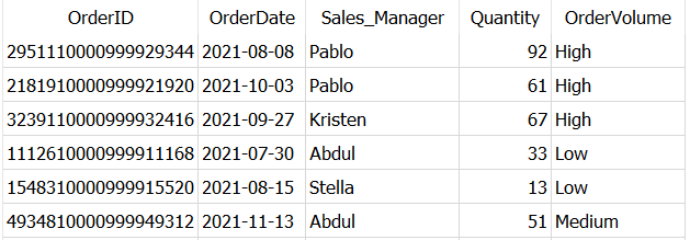
Simply, it created a new column OrderVolume and added values as ‘High’, ‘Low’, ‘Medium’ depending on the values in column Quantity.
📌 You can include multiple WHEN..THEN clauses and skip ELSE clause as it is optional.
📌 If you did not mention ELSE clause and no condition is satisfied, the query will return NULL for that specific record.
Another frequently used but lesser known use-case of CASE statement is — Data Pivoting.
Data pivoting is a process to rearrange the columns and rows in a result set so you can view data from different perspectives.
Sometimes the data you are dealing with is in long format (number of rows > number of columns) and you need to get it in wide format (number of columns > number of rows).
CASE statement comes handy in such situations. 💯
for example, let’s find out how many orders each sales manager handled for Singapore, UK, Kenya and India.
SELECT Sales_Manager,
       COUNT(CASE WHEN Shipping_Address = 'Singapore' THEN OrderID
             END) AS Singapore_Orders,

       COUNT(CASE WHEN Shipping_Address = 'UK' THEN OrderID
             END) AS UK_Orders,

       COUNT(CASE WHEN Shipping_Address = 'Kenya' THEN OrderID
             END) AS Kenya_Orders,

       COUNT(CASE WHEN Shipping_Address = 'India' THEN OrderID
             END) AS India_Orders
FROM Dummy_Sales_Data_v1
GROUP BY Sales_Manager
using CASE..WHEN..THEN we created separate columns for each of the shipping address to get the expected output as below.
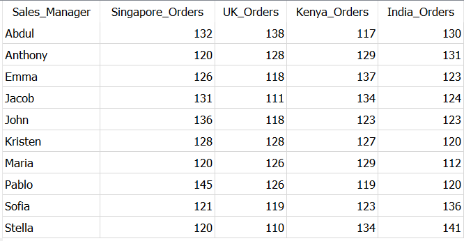
Depending on your use-case you can also use different aggregation such as SUM, AVG, MAX, MIN with CASE statement.
Next, when it comes to dealing real world data, it often contains date time values. Therefore it is important to understand how to extract different parts of date-time values such as month, week, year.
Extract Data From Date — Time Columns
In most of the interviews, you will be asked to aggregate the data month wise or calculate certain metric for a specific month.
And when there is no separate month column in the dataset, you need to extract required part of date out of date-time variable in data.
Different SQL environments have different functions to extract parts of a date. In general, in MySQL you should be aware of —
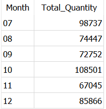
EXTRACT(part_of_date FROM date_time_column_name)YEAR(date_time_column_name)MONTH(date_time_column_name)MONTHNAME(date_time_column_name)DATE_FORMAT(date_time_column_name)for example, let’s find out total order quantity each month from Dummy Sales Dataset.
SELECT strftime('%m', OrderDate) as Month,
       SUM(Quantity) as Total_Quantity
from Dummy_Sales_Data_v1
GROUP BY strftime('%m', OrderDate)
If you are also using SQLite DB Browser like me, you have to use the function strftime() to extract the date parts as below. You need to use ‘%m’ in strftime() to extract month.
Below is a picture which shows most of the commonly extracted date parts, and keywords which you should use in EXTRACT function.
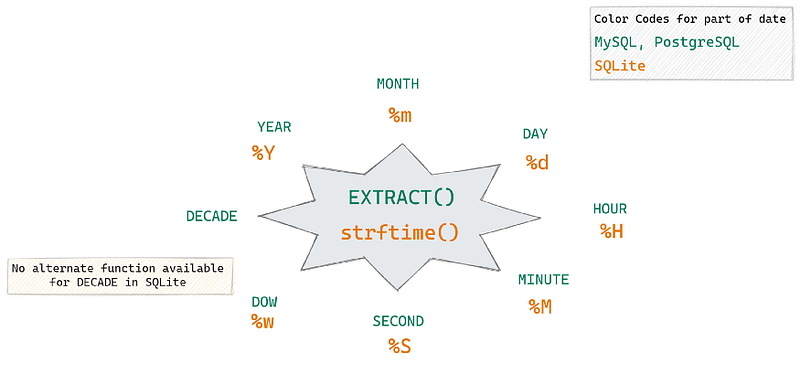
I explained almost all types of date part extraction in this quick read. Have a look at it to get a complete idea of it.
Last but not the least,
You’ll often see in real-world, data is stored in one large table rather than multiple small tables. That’s when SELF JOINs come into the picture to solve some of the interesting problems while working on these datasets.
SELF JOIN
These are exactly same as other JOINs in SQL, only difference is — in SELF JOIN you join a table with itself.
Remember, there is no SELF JOIN keyword, so you just use JOIN where both tables involved in the join are the same table. As both the table names are same, it is essential to use the table alias in case of SELF JOIN. ✅
Write a SQL query that finds out employees who earn more than their managers — One of the most frequently asked interview question on
SELF JOIN
let’s take this as example and create a Dummy_Employees dataset as below.
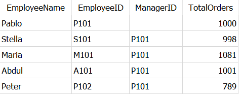
And try to get an find out which employees handle more orders than their manager using this query,
SELECT t1.EmployeeName, t1.TotalOrders
FROM Dummy_Employees AS t1
JOIN Dummy_Employees AS t2
ON t1.ManagerID = t2.EmployeeID
WHERE t1.TotalOrders > t2.TotalOrders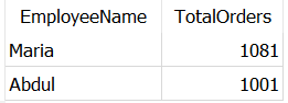
As expected, it returned employees — Abdul and Maria — who handled more orders than their manager — Pablo.
I get this question in almost 80% of the interviews I faced. So, it is the classic use-case of SELF JOIN.
That’s all!
I hope you finished this article quickly and found it useful to skill up SQL.
I’m using SQL since past 3 years, and I found these concepts often as interview questions for data analyst, data scientist positions. These concepts are very useful while working on real projects.
Interested in reading unlimited stories on Medium??
💡 Consider Becoming a Medium Member to access unlimited stories on medium and daily interesting Medium digest. I will get a small portion of your fee and No additional cost to you.
💡 Be sure to Sign-up to my Email list to never miss another article on data science guides, tricks and tips, SQL and Python.
Thank you for reading!


