A Complete Anomaly Detection Algorithm From Scratch in Python: Step by Step Guide

Anomaly Detection Algorithm Using the Probabilities

Anomaly detection can be treated as a statistical task as an outlier analysis. But if we develop a machine learning model, it can be automated and as usual, can save a lot of time. There are so many use cases of anomaly detection. Credit card fraud detection, detection of faulty machines, or hardware systems detection based on their anomalous features, disease detection based on medical records are some good examples. There are many more use cases. And the use of anomaly detection will only grow.

In this article, I will explain the process of developing an anomaly detection algorithm from scratch in Python.

The Formulas and Process

This will be much simpler compared to other machine learning algorithms I explained before. This algorithm will use the mean and variance to calculate the probability for each training data.

If the probability is high for a training example, it is normal. If the probability is low for a certain training example it is an anomalous example. The definition of high and low probability will be different for the different training sets. We will talk about how to determine that later.

If I have to explain the working process of anomaly detection, that’s very simple.

1. Calculate the mean using this formula:

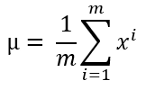
Here m is the length of the dataset or the number of training data and xi is a single training example. If you have several training features, most of the time you will have, the mean needs to be calculated for each feature.

2. Calculate the variance using this formula:

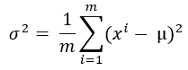
Here, mu is the calculated mean from the previous step.

3. Now, calculate the probability for each training example with this probability formula.

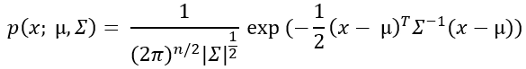
Don’t be confused by the summation sign in this formula! This is actually the variance in a diagonal shape.

You will see how it looks later when we will implement the algorithm.

4. We need to find the threshold of the probability now. As I mentioned before if the probability is low for a training example, that is an anomalous example.

How much probability is low probability?

There is no universal limit for that. We need to find that out for our training dataset.

We take a range of probability values from the output we got in step 3. For each probability, find the label if the data is anomalous or normal.

Then calculate precision, recall, and f1 score for a range of probabilities.

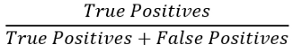
Precision can be calculated using the following formula

Recall can be calculated by the following formula:

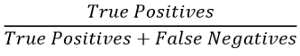
Here, True positives are the number of cases where the algorithm detects an example as an anomaly and in reality, it is an anomaly.

False Positives occur when the algorithm detects an example as anomalous but in the ground truth, it is not.

False Negative means the algorithm detects an example as not anomalous but in reality, it is an anomalous example.

From the formulas above you can see that higher precision and higher recall are always good because that means we have more true positives. But at the same time, false positives and false negatives play a vital role as you can see in the formulas as well. There needs to be a balance there. Based on your industry you need to decide which one is tolerable for you.

A good way is to take an average. There is a unique formula for taking an average. That’s called the f1 score. The formula for f1 score is:

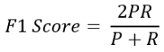
Here, P and R are precision and recall respectively.

I am not going into details on why the formula is that unique. Because this article is about anomaly detection. If you are interested in learning more about precision, recall, and f1 score, I have a detailed article on that topic here:

Based on the f1 score, you need to choose your threshold probability.

1 is the perfect f score and 0 is the worst probability score

Anomaly Detection Algorithm

I will use a dataset from Andrew Ng’s machine learning course which has two training features. I am not using a real-world dataset for this article because this dataset is perfect for learning. It has only two features. In any real-world dataset, it is unlikely to have only two features.

The good thing about having two features is you can visualize the data which is great for learners. Feel free to download the dataset from this link and follow along:

Let’s start the mission!

First, import the necessary packages

import pandas as pd 
import numpy as np

Import the dataset. This is an excel dataset. Here training data and cross-validation data are stored in separate sheets. So, let’s bring the training data.

df = pd.read_excel('ex8data1.xlsx', sheet_name='X', header=None)
df.head()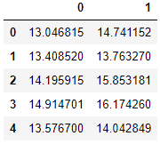

Let’s plot column 0 against column 1.

plt.figure()
plt.scatter(df[0], df[1])
plt.show()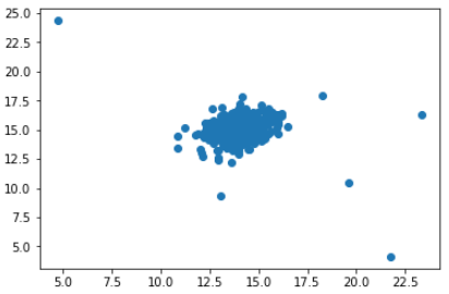

You probably know by looking at this graph which data are anomalous.

Check how many training examples are in this dataset:

m = len(df)

Calculate the mean for each feature. Here we have only two features: 0 and 1.

s = np.sum(df, axis=0)
mu = s/m
mu

Output:

0    14.112226
1    14.997711
dtype: float64

From the formula described in the ‘Formulas and Process’ section above, let’s calculate the variance:

vr = np.sum((df - mu)**2, axis=0)
variance = vr/m
variance

Output:

0    1.832631
1    1.709745
dtype: float64

Now make it diagonal shaped. As I explained in the ‘Formulas and Process’ section after the probability formula, that summation sign was actually the diagonals of the variance.

var_dia = np.diag(variance)
var_dia

Output:

array([[1.83263141, 0.        ],
       [0.        , 1.70974533]])

Calculate the probability:

k = len(mu)
X = df - mu
p = 1/((2*np.pi)**(k/2)*(np.linalg.det(var_dia)**0.5))* np.exp(-0.5* np.sum(X @ np.linalg.pinv(var_dia) * X,axis=1))
p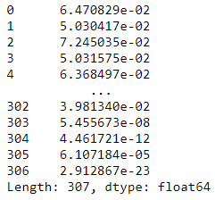

The training part is done.

Let’s put all these calculations for probability into a function for future use.

def probability(df):
    s = np.sum(df, axis=0)
    m = len(df)
    mu = s/m
    vr = np.sum((df - mu)**2, axis=0)
    variance = vr/m
    var_dia = np.diag(variance)
    k = len(mu)
    X = df - mu
    p = 1/((2*np.pi)**(k/2)*(np.linalg.det(var_dia)**0.5))* np.exp(-0.5* np.sum(X @ np.linalg.pinv(var_dia) * X,axis=1))
    return p

The next step is to find out the threshold probability. If the probability is lower than the threshold probability, the example data is anomalous data. But we need to find out that threshold for our particular case.

For this step, we use cross-validation data and also the labels. In this dataset, we have the cross-validation data and also the labels in separate sheets.

For your case, you can simply keep a portion of your original data for cross-validation.

Now import the cross-validation data and the labels:

cvx = pd.read_excel('ex8data1.xlsx', sheet_name='Xval', header=None)
cvx.head()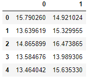

Here are the labels:

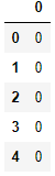
cvy = pd.read_excel('ex8data1.xlsx', sheet_name='y', header=None)
cvy.head()

The purpose of cross-validation data is to calculate the threshold probability. And we will use that threshold probability to find the anomalous data of df.

Now call the probability function we defined before to find the probability for our cross-validation data ‘cvx’:

p1 = probability(cvx)

I will convert ‘cvy’ to a NumPy array just because I like working with arrays. DataFrames are also fine though.

y = np.array(cvy)

Output:

#Part of the array
array([[0],
       [0],
       [0],
       [0],
       [0],
       [0],
       [0],
       [0],
       [0],

Here, the value of ‘y’ 0 suggests that that’s a normal example, and the ‘y’ value of 1indicates that, it is an anomalous example.

Now, how to select a threshold?

I do not want to just check for all the probability from our list of probability. That may be unnecessary. Let’s examine the probability values some more.

p.describe()

Output:

count    3.070000e+02
mean     5.378568e-02
std      1.928081e-02
min      1.800521e-30
25%      4.212979e-02
50%      5.935014e-02
75%      6.924909e-02
max      7.864731e-02
dtype: float64

As you can see in the picture, we do not have too many anomalous data. So, if we just start from the 75% value, that should be good. But just to be extra safe I will start the range from the mean.

So, we will take a range of probabilities from the mean value and lower. We will check the f1 score for each probability of this range.

First, define a function to calculate the true positives, false positives, and false negatives:

def tpfpfn(ep, p):
    tp, fp, fn = 0, 0, 0
    for i in range(len(y)):
        if p[i] <= ep and y[i][0] == 1:
            tp += 1
        elif p[i] <= ep and y[i][0] == 0:
            fp += 1
        elif p[i] > ep and y[i][0] == 1:
            fn += 1
    return tp, fp, fn

Make a list of the probabilities that are lower than or equal to the mean probability.

eps = [i for i in p1 if i <= p1.mean()]

Check, the length of the list,

len(eps)

Output:

128

Define a function to calculate the ‘f1’ score as per the formula we discussed before:

def f1(ep, p):
    tp, fp, fn = tpfpfn(ep)
    prec = tp/(tp + fp)
    rec = tp/(tp + fn)
    f1 = 2*prec*rec/(prec + rec)
    return f1

All the functions are ready!

Now calculate the f1 score for all the epsilon or the range of probability values we selected before.

f = []
for i in eps:
    f.append(f1(i, p1))
f

Output:

[0.16470588235294117,
 0.208955223880597,
 0.15384615384615385,
 0.3181818181818182,
 0.15555555555555556,
 0.125,
 0.56,
 0.13333333333333333,
 0.16867469879518074,
 0.12612612612612614,
 0.14583333333333331,
 0.22950819672131148,
 0.15053763440860213,
 0.16666666666666666,
 0.3888888888888889,
 0.12389380530973451,

This is a part of the f score list. The length should be 128. The f scores are usually ranged between 0 and 1 where 1 is the perfect f score. The higher the f1 score the better. So, we need to take the highest f score from the list of ‘f’ scores we just calculated.

Now, use the ‘argmax’ function to determine the index of the maximum f score value.

np.array(f).argmax()

Output:

127

And now use this index to get the threshold probability.

e = eps[127]
e

Output:

0.00014529639061630078

Find out the Anomalous Examples

We have the threshold probability. We can find out the labels of our training data from it.

If the probability value is lower than or equal to this threshold value, the data is anomalous and otherwise, normal. We will denote the normal and anomalous data as 0and 1 respectively,

label = []
for i in range(len(df)):
    if p[i] <= e:
        label.append(1)
    else:
        label.append(0)
label

Output:

[0,
 0,
 0,
 0,
 0,
 0,
 0,
 0,
 0,
 0,

This is part of the label list.

I will add these calculated labels in the training dataset above:

df['label'] = np.array(label)
df.head()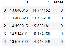

I plotted the data where the label is 1 in red color and where the label is zero in black. Here is the plot.

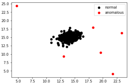
Does it make sense?

It does, right? The data in red are clearly anomalous.

Conclusion

I tried to explain the process to develop an anomaly detection algorithm step by step. I did not leave any steps hidden here. I hope it is understandable. If you are having trouble understanding just by reading it, I suggest run every piece of code by yourself in a notebook. That will make it very clear.

Please do not hesitate to share, if you are doing some cool projects using this algorithm.

Feel free to follow me on Twitter and like my Facebook page.