3D Python

3D Model Fitting for Point Clouds with RANSAC and Python

A 5-Step Guide to create, detect, and fit linear models for unsupervised 3D Point Cloud binary segmentation: RANSAC implementation from scratch.

Have you ever wondered why we find so much geometry in the world surrounding us? No, you did not? Good news, it means you are sane. I tend to have weird interrogations about life and stuff 🙃. I find it so fascinating, Especially the symmetrical wonders of ❄️ flakes, the elementary shapes in tasty🍈, or the wonders of heritage design 🕌 patterns.

Our world is filled with different geometrical flavors. But if you look around, I bet you can find at least five simple geometries. We notice that most of the shapes we find can be tied to geometric primitives such as planes, pyramids, cylinders, cubes, and spheres. And this is a compelling observation; why?

Let us assume we can capture and then digitize our real-world environment in great detail. Would it not be convenient to detect within these 3D digital replicas which shapes are composing the scene and use that as a layer for semantic extraction? For modeling? For scene understanding?

Haha, precisely! In this tutorial, I will give you a swift way to define 3D planes and use them as a base to partition 3D Point Clouds.

And for this, we will cover a robust algorithm and implement it from scratch: RANSAC! Are you pumped and ready? Let us dive in!

Step 0. The Strategy

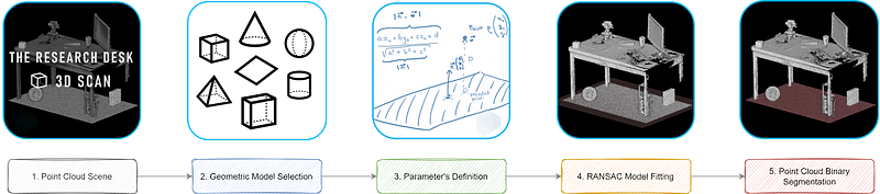
Before bluntly approaching the project with an efficient solution, let us frame the overall approach. This tutorial follows a strategy comprising five straightforward steps, as illustrated in our strategy diagram below.

First, (1) we chose a point cloud dataset among the three I share with you. Then, (2) we select one geometric model to detect in the data. (3) The definition of the parameters to generalize is studied. (4) we mix’n’match these three ingredients with the RANSAC recipe, (5) we segment our point cloud(s): et voilà! A nicely cooked point cloud! The strategy is laid out, and below, you can find the quick links to the steps:

Step 1. The Point Cloud Data
Step 2. Geometric Model Selection
Step 3. Parameter's Definition
Step 4. RANSAC Model Fitting (from scratch)
Step 5. Point Cloud Binary Segmentation

Perspectives & Conclusion

Now that we are set up, let us jump right in.

Step 1. The Point Cloud Data

All right, let us get going. We will design a method that is easily extendable to different use cases. For this purpose, it is not one but three datasets that you have the option to choose from, download, and do your scientific experiments on 😁. These were chosen to illustrate three different scenarios and provide the base data to play with. How cool, hun?

The scenarios that we will want to showcase are the following:

• 🤖 ROBOTICS: We are designing a robot that needs to clean both the ground and the table and make sure to avoid obstacles when cleaning. On top, we will want to detect the position of elements of interest and use that as a basis for future cleaning tasks to know if we need to reposition them initially.
• 🚙 ADAS (Advanced Driver-Assistance System): Here, we are interested in giving a vehicle the ability to drive by itself: an Autonomous Vehicle. For this purpose, we use one epoch of a Velodyne VLP-16 scan, on which we usually do real-time analysis for object detection.
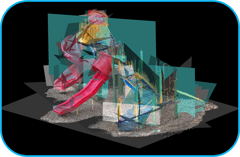
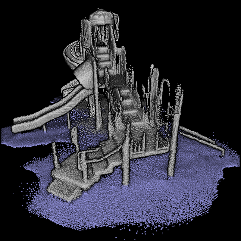
• 🏚️ CONSTRUCTION: A Playground constructed some years ago presents problems due to an unstable groundwork. Therefore, we want to assess the planarity of the element and determine if a leveling operation is necessary.

To ensure your choice, you can play with them online with the Flyvast WebGL App and then download them here (The Researcher Desk (.xyz), The Car (.xyz), The Playground (.xyz)).

Step 2. Choosing a Geometric Model

In a previous article that proposed to automate both segmentation and clustering, we defined the RANSAC approach:

RANSAC (RANdom SAmple Consensus) is a kind of trial-and-error approach that will group your data points into two segments: an inlier set and an outlier set.

To achieve this goal, we proceed in three straightforward steps:

• We choose a geometric model that fits a tiny random sample from our dataset (3 points taken randomly if we want to define a plane).
• We then estimate how good the fit is by checking how many points are “close” to the surface of interest, and thus we get an inlier count.
• We repeat this process over a certain amount of iterations and keep the plane that maximizes the inlier count.

The approach is not rocket science but a super-practical approach for noisy, real-world datasets.

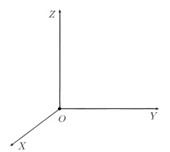
In this tutorial, we chose: plane geometry! It is the best way to quickly make sense of the extensive array of datasets out there. But bear with me; I will now give you some crucial mathematical understanding we use to describe a plane in Euclidean Space. The general form of the equation of a plane in ℝ³ is 𝑎𝑥+𝑏𝑦+𝑐𝑧+𝑑=0.

What a beauty 🦋. Laughing aside, the 𝑎,𝑏, and 𝑐 constants are the components of the normal vector ñ=(𝑎,𝑏,𝑐), which is perpendicular to the plane or any vector parallel to the plane. When you grasp this, playing around with transformations (translations, rotations, scaling) and fitting it is super easy. The d constant will shift the plane from the origin.

It means that a point p = (𝑥,𝑦,𝑧) belongs to the plane guided by the normal vector ñ, if it satisfies the equation. If you understand this, you get the first-hand principle that guides geometric fitting. Great!

Now let us fit planes everywhere with RANSAC.

The RANSAC Soup, isn’t it? Okay, let us define the parameters to make it work properly.

Step 3. Parameter’s Definition

It is time to dirty our undersized coder's hands! And this time, let us code a RANSAC Plane Detection Algorithm for Point Clouds from scratch to grasp better what is under the hood. We will do this with two libraries: random and numpy. Hard to be more minimalistic. And for visualization, our beloved (or sweet enemy 😊) matplotlib and also plotly for interactive Jupyter notebooks and the Google Colab Script.

import random
import numpy as np
import matplotlib.pyplot as plt
from mpl_toolkits import mplot3d

import plotly.express as px

A. Choose a dataset wisely

What is your weapon of choice? I will take my research desk as the main case study:

dataset="the_researcher_desk.xyz"
pcd = np.loadtxt(data_folder+dataset,skiprows=1)

I then prepare it quickly by separating the geometric attribute from the radiometric ones:

xyz=pcd[:,:3]
rgb=pcd[:,3:6]

Okay, now it is time to cook some parameters.

B. Manual parameters set-up

We need to define a threshold parameter to determine whether a point belongs to the fitted planar shape (inlier) or is an outlier. We will base our discrimination on a point-to-plane distance; we thus need to grasp the unit in our point cloud quickly. Let us display the point cloud with matplotlib:

plt.figure(figsize=(8, 5), dpi=150)
plt.scatter(xyz[:,0], xyz[:,1], c=rgb/255, s=0.05)
plt.title("Top-View")
plt.xlabel('X-axis (m)')
plt.ylabel('Y-axis (m)')
plt.show()

Sometimes, it can be hard to decipher what separates two points, especially using Google Colab and non-interactive renders. If you are in such a scenario, you can use plotly with import plotly.express as px, and then you can get the figure with

fig = px.scatter(x=xyz[:,0], y=xyz[:,1], color=xyz[:,2])
fig.show()

It allows us to see that, on average, neighboring points every 5 mm, thus we set the threshold parameter ten times higher (absolutely empirical 😊): threshold=0.05. In this same vein, we will set up the number of iterations to a considerable number not to be limited; let us say 1000 iterations:

iterations=1000

C. Automatic parameters set-up

We may be a bit limited by needing some domain knowledge to set up the threshold. Therefore, it would be exciting to try and bypass this to open the approach to non-experts. I will share with you a straightforward thought that could be useful. What if we were to compute the mean distance between points in our datasets and use this as a base to set up our threshold?

Well, it is an idea worth exploring. To try and determine such a value, we could use a KD-Tree to speed up the process of querying the nearest neighbors for each point. At this stage of the process, I recommend using scikit-learn implementation and separating into two hyperplanes the KD-tree at each node:

from sklearn.neighbors import KDTree
tree = KDTree(np.array(xyz), leaf_size=2)  

From there, we can then query the k-nearest neighbors for each point in the point cloud with the simple query method:

tree.query(xyz, k=8)

Which outputs the point distance and the point indexes, respectively:

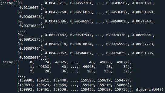
🤓 Note: the first distance value of the nearest neighbor is all the time equal to 0. Weird, you ask? This is because we query the whole point cloud against itself; thus, each point has a distance to itself. Therefore, we need to filter the first element per row: nearest_dist, nearest_ind = tree.query(xyz, k=8)

Great! So now, if we average over each neighbor candidate, sorted from the closest to the farthest with np.mean(nearest_dist[:,1:],axis=0), we obtain:

>> array([0.0046, 0.0052 , 0.0059, 0.0067, 0.0074, 0.0081, 0.0087])

It means that if we reasoned by considering the nearest neighbor, we would have an average distance of 4.6 mm. If we were in a scenario where we wanted to get a local representation of the mean distance of each point to its nth closest neighbors, using np.mean(nearest_dist[:,1:]), outputs 6.7 mm in our case.

To get something running smoothly for your experiments, I recommend setting a query using between 8 to 15 points taken as neighbors and averaging on it. It thus gives a good local representation of the noise ratio in the point cloud. We will explore more ingenious ways to find the noise ratio of a point cloud in future tutorials. 😉

🧙‍♂️ Experts: There exists an automatic way to get the iteration number right every time. If we want to succeed with a probability p (e.g., 99%), the outlier ratio in our data is e (e.g., 60%), and we need s point to define our model (here 3). The formula below gives us the number of trials (iterations) to make:

Step 4. Model fitting with RANSAC

A. Finding a plane (1 Iteration)

Let us simulate an iteration before automating over the specified number in iterations.

First off, we will want to grasp three random points from the point cloud:

idx_samples = random.sample(range(len(xyz)), 3)
pts = xyz[idx_samples]

Then, we want to determine the equation of the plane. e.g., finding the parameters 𝑎,𝑏,𝑐, and 𝑑 of the equation 𝑎𝑥+𝑏𝑦+𝑐𝑧+𝑑=0. For this, we can play with a fantastic linear algebra property that says that the cross product of two vectors generates an orthogonal one.

We thus just need to define two vectors from the same point on the plane vecA and vecB, and then compute the normal to these, which will then be the normal of the plane. How awesome is that?

vecA = pts[1] - pts[0]
vecB = pts[2] - pts[0]
normal = np.cross(vecA, vecB)

From there, we will normalize our normal vector, then get 𝑎,𝑏, and 𝑐 that define the vector, and find 𝑑 using one of the three points that fall on the plane: d = — (𝑎𝑥+𝑏𝑦+𝑐𝑧)

a,b,c = normal / np.linalg.norm(normal)
d=-np.sum(normal*pts[1])

And now, we are ready to attack the computation of any remaining point to the plane we just defined 💪.

B. Point-to-Plane Distance: The threshold definition

If you are up taking my word for it, here is what we need to implement:

This distance is the shortest, being the orthogonal distance between the point and the plane, as illustrated below.

It means that we can simply compute this distance by taking each point in the point cloud that is not part of the three ones that we used to establish a plane in one Ransac iteration, just like this:

distance = (a * xyz[:,0] + b * xyz[:,1] + c * xyz[:,2] + d
            ) / np.sqrt(a ** 2 + b ** 2 + c ** 2)

Which, for our random choice and plane fit outputs:

array([-1.39510085, -1.41347083, -1.410467 , …, -0.80881761, -0.85785174, -0.81925854])

🤓 Note: see the negative values? We will have to address this to get unsigned distances because our normal is flippable 180° on the plane.

Very nice! From there, we can just check against the threshold and filter all points that answer the criterion to only keep as inliers the points with a point-to-plane distance under the threshold.

idx_candidates = np.where(np.abs(distance) <= threshold)[0]

🤓 Note: the [0] allows us to only work with indexes at this step, not to overflow our system with unnecessary point coordinates.

Do you already know what the next sub-step will be about? 🤔

C. Iteration and function definition

Indeed, we now need to iterate a certain amount to find the optimal plane! For this purpose, we will define a function that takes as an input point coordinates, the threshold, and the number of iterations, and return the plane equation and the point inliers indexes with:

def function(coordinates, threshold, iterations):
  ...
  i=1
  while i < iterations:
    do <<all below>>
    if len(idx_candidates) > len(inliers):
      equation = [a,b,c,d]
      inliers = idx_candidates
    i+=1
  return equation, inliers

🤓 Note: we create the RANSAC loop over the iteration parameter. For each loop, we will compute the best fitting RANSAC plane, and retain both the equation and the inliers indexes. With the if statement, we then check if the score of the current iteration is the biggest, in which case we switch the point indexes.

Now, let us fill our RANSAC function and get the following:

def ransac_plane(xyz, threshold=0.05, iterations=1000):
  inliers=[]
  n_points=len(xyz)
  i=1

  while i<iterations:
    idx_samples = random.sample(range(n_points), 3)
    pts = xyz[idx_samples]

    vecA = pts[1] - pts[0]
    vecB = pts[2] - pts[0]
    normal = np.cross(vecA, vecB)
    a,b,c = normal / np.linalg.norm(normal)
    d=-np.sum(normal*pts[1])

    distance = (a * xyz[:,0] + b * xyz[:,1] + c * xyz[:,2] + d
                ) / np.sqrt(a ** 2 + b ** 2 + c ** 2)

    idx_candidates = np.where(np.abs(distance) <= threshold)[0]

    if len(idx_candidates) > len(inliers):
      equation = [a,b,c,d]
      inliers = idx_candidates
    
    i+=1
  return equation, inliers

And here we are, we created a RANSAC function for plane detection that eats 3D point clouds !!!! It is sufficiently optimized in this way for you to attack big point clouds without the risks of your computer burning 🔥! Now, let us extend to the practical case where we want to segment our point cloud.

Step 5. Point Cloud Binary Segmentation

This is the final step! At least for this stage 😀. We will retain the results of the function in two variables:

eq,idx_inliers=ransac_plane(xyz,0.01)
inliers=xyz[idx_inliers]

Very nice! But now, we also want to split the original point cloud and grasp the outliers efficiently. Here is an excellent turnaround. We create a mask that will act as a quick filter to get the rest of the points that do not belong to inliers:

mask = np.ones(len(xyz), dtype=bool)
mask[idx_inliers] = False
outliers=xyz[mask]

Superb! We now have an inlier set and an outlier set! Let us check out the results with matplotlib:

ax = plt.axes(projection='3d')
ax.scatter(inliers[:,0], inliers[:,1], inliers[:,2], c = 'cornflowerblue', s=0.02)
ax.scatter(outliers[:,0], outliers[:,1], outliers[:,2], c = 'salmon', s=0.02)
plt.show()

Wow, it works very nicely! We found the ground in this scene! How awesome! Last thing: Exporting both datasets independently:

result_folder=”../DATA/RESULTS/”
np.savetxt(result_folder+dataset.split(“.”)[0]+”_inliers.xyz”, inliers, fmt=’%1.4f’, delimiter=’;’)
np.savetxt(result_folder+dataset.split(“.”)[0]+”_outliers.xyz”, outliers, fmt=’%1.4f’, delimiter=’;’)

And what about the other datasets? Here are the results we get by using the automatic thresholding method, based on a distance estimation to the 15-th nearest neighbors! How nice!

It is fascinating that we are super robust to noise and data context! You deserve the complete code accessible and runnable on this Google Colab Notebook. Enjoy!

Conclusion

Bravo 🥳! You implemented a complete RANSAC Model Fitting Algorithm for Plane Detection and 3D Point Cloud Segmentation from scratch. On top, you can now automatically set RANSAC Parameters so that you have not a 99% automatic solution but a 100% Automation. And this is a significant step! If you want to dive deeper and check out how to include this new skill in your project, below is the next-step tutorial that will allow you to iterate the RANSAC method and use clustering approaches to detect instances in your point cloud:

My contributions aim to condense actionable information so you can start from scratch to build 3D automation systems for your projects. You can get started today by taking a course at the Geodata Academy.

Going Further

Other advanced segmentation methods for point clouds exist. It is a research field in which I am deeply involved, and you can already find some well-designed methodologies in the articles [1–6]. For the more advanced 3D deep learning architectures, some comprehensive tutorials are coming very soon!

1. Poux, F., & Billen, R. (2019). Voxel-based 3D point cloud semantic segmentation: unsupervised geometric and relationship featuring vs. deep learning methods. ISPRS International Journal of Geo-Information. 8(5), 213; https://doi.org/10.3390/ijgi8050213 — Jack Dangermond Award (Link to press coverage)
2. Poux, F., Neuville, R., Nys, G.-A., & Billen, R. (2018). 3D Point Cloud Semantic Modelling: Integrated Framework for Indoor Spaces and Furniture. Remote Sensing, 10(9), 1412. https://doi.org/10.3390/rs10091412
3. Poux, F., Neuville, R., Van Wersch, L., Nys, G.-A., & Billen, R. (2017). 3D Point Clouds in Archaeology: Advances in Acquisition, Processing and Knowledge Integration Applied to Quasi-Planar Objects. Geosciences, 7(4), 96. https://doi.org/10.3390/GEOSCIENCES7040096
4. Poux, F., Mattes, C., Kobbelt, L., 2020. Unsupervised segmentation of indoor 3D point cloud: application to object-based classification, ISPRS — International Archives of the Photogrammetry, Remote Sensing and Spatial Information Sciences. pp. 111–118. https://doi:10.5194/isprs-archives-XLIV-4-W1-2020-111-2020
5. Poux, F., Ponciano, J.J., 2020. Self-learning ontology for instance segmentation of 3d indoor point cloud, ISPRS — International Archives of Photogrammetry, Remote Sensing and Spatial Information Sciences. pp. 309–316. https://doi:10.5194/isprs-archives-XLIII-B2-2020-309-2020
6. Bassier, M., Vergauwen, M., Poux, F., (2020). Point Cloud vs. Mesh Features for Building Interior Classification. Remote Sensing. 12, 2224. https://doi:10.3390/rs12142224