Summary

The article introduces three fundamental Google Sheets tools—text wrapping, the =SUM() function, and conditional formatting—to enhance spreadsheet management for beginners.

Abstract

The article "3 Lifechanging Google Sheets Tools for Complete Beginners" provides a guide to essential features within Google Sheets that can significantly improve the user experience for those new to the software. The author emphasizes the practicality of these tools by using a weekly meal plan as a relatable example, demonstrating how text wrapping can clean up cell presentation, the =SUM() function can simplify calculations, and conditional formatting can highlight important data points. By focusing on these tools, the author aims to demystify the complexity often associated with spreadsheets and encourage users to embrace them for personal or professional use.

Opinions

The author initially found spreadsheets confusing and clunky but gained a new appreciation for them after learning proper techniques.
Text wrapping is presented as a straightforward solution to the common issue of text overflow in cells, enhancing readability.
The =SUM() function is highlighted as a versatile and indispensable tool for calculations within Google Sheets.
Conditional formatting is considered an advanced but valuable feature for drawing attention to specific data, such as empty cells or values outside a desired range.
The author believes that mastering these tools can transform one's approach to spreadsheet software and potentially have a life-changing impact.

3 Lifechanging Google Sheets Tools for Complete Beginners

Read about the Google Sheets tools that everyone should know (not just data analysts)!

When I sat down to write this tutorial I originally planned on pulling up a spreadsheet example that I had made for my data analytics class. The spreadsheet I first pulled up was in Google Sheets and dealt with a dataset about a fictional grocery stores monthly sales. Then I realized that that's not relatable to the average person. So instead for this tutorial we will be using my weekly meal plan. I’ll show you in a few steps how I use 3 simple but powerful tools to save me time and work!

In the last few years working in a STEM field with an interest in data I’ve learned to have a new appreciation for spreadsheets. I used to hate the endless “=FORMULAS” of Excel and Google Sheets finding them confusing and clunky. It wasn’t until I started using Google Sheets for data analytics that I learned why I hated them. I was doing it wrong!

The truth is that you don’t need to learn fancy formulas to upgrade your game in Google Sheets. A few easy to use but powerful tools is enough to completely change your relationship with spreadsheet software and maybe even change your life…

1. Text Wrapping

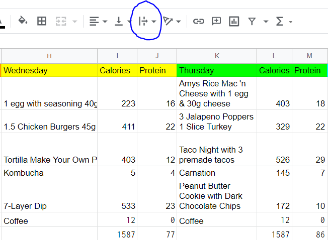
Image by author with the help of Google Sheets

Can anyone even tell me what meal is in cell H4 on the Wednesday part of the meal plan? Or any meal on Wednesday? Exactly.

How about Thursdays meals? These are a lot better. That’s because Thursdays meals are formatted with something called: text wrapping.

For anyone who doesn’t use Google Sheets too often and has to use it for work or school I can empathize with why Google Sheets might drive them nuts. I remember at one of my old jobs the first time I had to start a new Google Sheet for customer sales and all the customers names overflowed the cells into neighboring cells. It drove me nuts! Luckily text overflow is an easy problem to solve with text wrapping.

First highlight the cells or cell that you want to apply text wrapping too.

Then simply find and click the text wrapping button in Google Sheets. Its circled in the above image in blue!

Once you click the text wrapping button it will reveal a toolbar that looks like this:

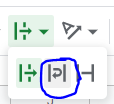
Again click the button circled in blue. This is the wrap button. Now your cells should look like Thursdays meals not Wednesdays!

2. =Sum

Okay I know, I said that you don’t need a bunch of fancy formulas to change how to use Google Sheets… and I really do believe that. Its true.

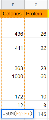
But =SUM() is a classic. Probably about 90% of the time I need to calculate something in a spreadsheet or get important information from it I use =SUM().

=SUM() is exactly what it sounds like: it summarizes things. To use this function simply type in a cell

=SUM(*data to summarize*)

=SUM() takes input in the form of multiple cells added together, a range of rows/columns or even a single column. In case you don’t know Google Sheets has uses the column headings (letters) + the row headings (numbers) in order to identify specific cells. Here are some examples of =SUM() in action:

Multiple Cells Added Together

=SUM(A1, B8, J2) or =SUM(A1+B8+J2)

A Range of Rows or Columns

=SUM(A1:A8)

A Single Cell

=SUM(A6)

3. Conditional formatting

Conditional formatting is definitely the most advanced out of these 3 tools but in my opinion its worth a little extra effort to learn. After all once you learn it you will have that skill forever!

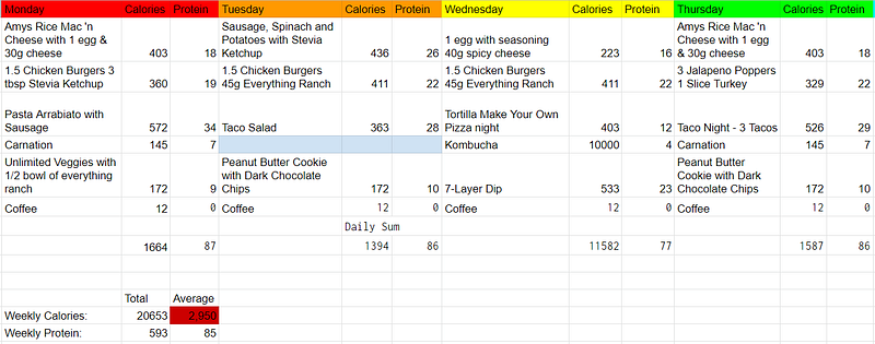
Note the red and blue cells on the spreadsheet! These cells are using conditional formatting to bring an issue to my attention. In the meal plan section I use conditional formatting to change the color of any cell that is empty to a light blue. This way if I forget to fill something out it jumps out at me and brings my attention to it more than just a blank cell. Finding blank cells is probably what I use conditional formatting for the most.

You can also use conditional formatting for other types of checks. In the example above, my daily average of calories is 2,950 so I have Google Sheets highlight the cell in red to bring that to my attention because that’s well over my caloric goals.

How to Use Conditional Formatting

To use conditional formatting in Google Sheets click on a cell or highlight the range of cells that you want to apply conditional formatting to. Then right click to bring up the menu depicted below.

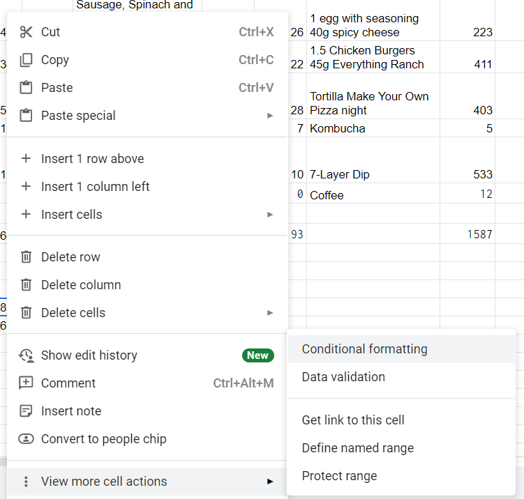
Hover your mouse over “View more cell actions” to bring up another submenu. Click on “Conditional formatting” to bring up the Conditional Format Rules section on the right side of the screen.

It will look like this:

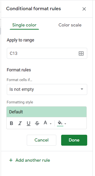
There are 3 sections of the Conditional Format Rules section to be aware of for simple conditional formatting: the range, the if condition (Format cells if…) and the formatting style.

The range is the cell or cells that you highlighted earlier.

The if condition (Format cells if…) is the rule for formatting. You can use this to check if cells are empty, if they contain certain values, if they are equal to certain or if they are greater than/less than certain values.

Formatting style is the change that the spreadsheet will apply if the if condition is met. This is typically a color. I like to use lighter colors for checking if cells are empty and darker colors for everything else.

In Conclusion

Now you’ve learned 3 new tools for Google Sheets!

Remember if you forget anything you can always check back with this article. In the meantime, happy spreadsheeting!