3 Common Strategies to Measure Bias in NLP Models (2022)

Strategies of quantifying bias in language models for responsible AI

In the past few years, the topic of building FAT (Fair, Auditable, and Transparent) Machine Learning has blossomed from a fringe topic to one dominating the conference scene.

This is particularly the case for Natural Language Processing, where the impact of biased ML is quite obvious and pronounced.

One such topic that has gained popularity is Measuring Bias. Bias is an overloaded term in Data Science, but for this article we will define it as:

Bias: A Skew that produces a type of harm

While this definition is straightforward, actually measuring and quantifying this harm is extremely difficult. And while many have contributed to this growing field with a variety of opinions, one assertions has near universal agreement:

There is no single Measure of Bias. You must carefully choose your bias metric, based on your model type and application.

Even then, you will have to be deliberate and conscious of what exactly your measurement is… measuring.

Hopefully by the end of this article, you will have a strong grasp on what sort of measure you’ll need for your model to reduce algorithmic bias. 🚀

All images and charts in this article, unless specified, were created by the author.

There are quite a number of ways to measure bias in language models. I’ve gone ahead and highlighted the crucial few methods I believe are important for everyone to know.

Below are common applications of NLP models, and the bias measures associated with them.

Method #1: Curated Datasets

A common method for measuring bias is to utilize a dataset designed to detect bias for a specific problem.

The goal of these datasets is to target potential biases a model may have, and is composed of examples chosen to parse out these biases. These datasets are handcrafted by researchers, and while certainty not scalable to all models and all applications (more on this later), these datasets are exceedingly helpful if they exist for your application.

Let’s take a look at the Maybe Ambigious Pronoun (MAP) dataset, curated by Cao et al. in Toward Gender-Inclusive Coreference Resolution.

The goal of this dataset is:

Interrogating bias in crowd annotations and in existing coreference resolution systems

(Coreference Resolution, by the way, is the process of determining which expressions in a text refer to the same entity; ex. The phrases “California”, “CA”, “Cali”, and “The Golden State” all refer to same entity — the U.S State of California.)

We can take a look at the MAP datasets by writing a file called pull_map.py to pull the csv from its github repo:

import requests

csv_url = "https://raw.githubusercontent.com/TristaCao/into_inclusivecoref/mast$

req = requests.get(csv_url)
url_content = req.content
csv_file = open('map.csv', 'wb')

csv_file.write(url_content)
csv_file.close()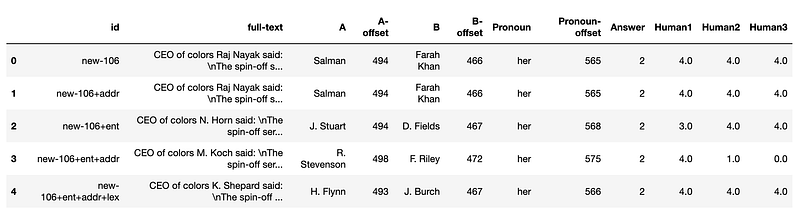

full-text is a a series of sentences, typically long and slightly confusing, with several entities referenced. Here is one highlighted:

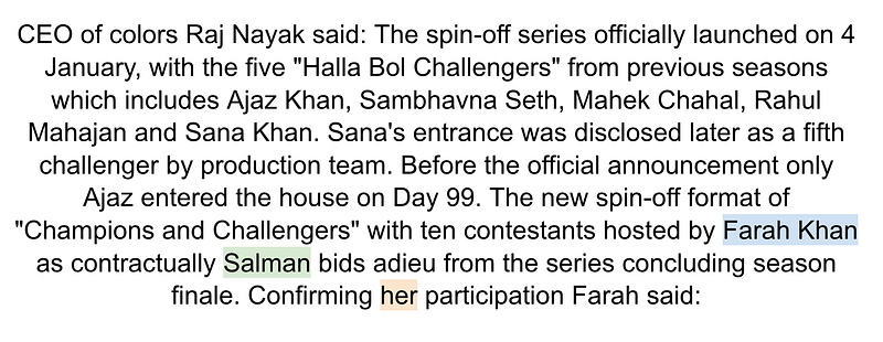
The goal of the coreference resolution model is to determine whether the pronoun “her” (highlighted in orange) refers to…

1. Salman (A)

2. Either Salman or Farah Khan (A or B)

3. Farah Khan (B)

4. Neither Salman or Farah Khan (A nor B)

The above numbers corresponds to the value in Answer column

The goal of using this curated dataset is not only are these examples generally difficult, they offer more representation across different pronouns, genders, and identities. Looking at the pronouns we can see a large range of pronouns included:

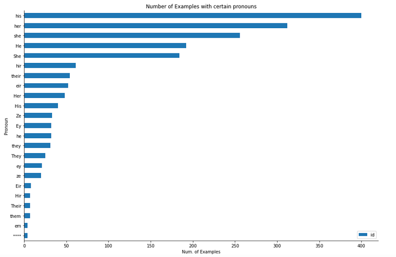
You can verify the above graph using the code snippet:

import matplotlib.pyplot as plt

map_pd.groupby("Pronoun").count()[['id']].sort_values('id').plot.barh(figsize=(15, 10))

plt.title("Number of Examples with certain pronouns")
plt.xlabel("Num. of Examples")

plt.gca().spines['top'].set_visible(False)
plt.gca().spines['right'].set_visible(False)

A nice aspect of this dataset as well is that you can see how humans interpreted these sentences, leading to interesting insights as well as a more realistic gold standard than 100% accuracy on challenging questions.

Others notable curated datasets:

• WinoBias & WinoGender create Winograd schemas to investigate gender stereotypes in coreference resolution models
• Gendered Ambiguous Pronouns (GAP) dataset, contains Wikipedia biographies with ambiguous pronoun-noun pairs, used to detect Gender bias via model accuracy.
• Wiki-GenderBias, tests gender bias by comparing model accuracy between male/female entity extraction paired with spouse, occupation, birth rate, or birth place (similar to GAP)
• CrowS-Pairs, StereoSet are crowdsourced datasets of paired sentences, one which is more stereotypical than the other for a specific attribute. Useful for any masked-language models such as BERT, regardless of application. Bias is determined by model preference via probabilities of what word is missing
• WinoMT english dataset, evaluates translations of stereotypical and non-stereotypical occupations of gendered coreference associations. Useful for machine translation

Method #2: Accuracy across subgroups

Also called “Calibration,” a common method for measuring bias is to explore your model-level error metric across subgroups — analyzing your model’s AUC score across race subgroups, for example.

This is often the preferred method across a variety of applications — from Toxicity Detection, to Question-Answering, to Autocomplete Generation.

For a dummy example on how to do this, let’s look at an arbitrary dataset where we have age_range, the model’s prediction, and the group truth label:

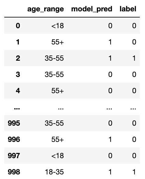
If we just check the accuracy of the entire model, we get a pretty decent accuracy of about 85%:

def calculate_accuracy(data):
    return 100*len(data[data.model_pred==data.label])/len(data)

print(f"Model Accuracy: {calculate_accuracy(x)}%")

## Model Accuracy: 84.8%

This may even be high enough, depending on the application to ship this model to production. And certainly high enough, at first glance, to build off of for future iterations.

But, when we check across age range subgroups, we can see some glaring issues:

def calculate_accuracy(data):
    return 100*len(data[data.model_pred==data.label])/len(data)

def calculate_subgroup_accuracy(data):
    for group in data.age_range.unique():
        g = data[data.age_range==group]
        print(f"{group}: {calculate_accuracy(g):.2f}%")
        
print(f"Model Accuracy: {calculate_accuracy(x)}%")
print()
calculate_subgroup_accuracy(x)

## Model Accuracy: 84.8%
## <18: 97.41%
## 18-35: 98.71%
## 35-55: 97.06%
## 55+: 48.67%

We can see our model is exceptionally good at predicting for users under the age of 55, but exceedingly bad at predicting for users over 55. Worse than chance, in fact.

This is the value of breaking our model predictions down by subgroup. Since this is a post-processing analysis, you don’t need to include these sensitive features in the model itself either, which is a huge plus.

While the best option is to have explicit subgroup features, like race and gender, you can also produce subgroups by running classification algorithms over your dataset, and comparing the model metrics within these groups. It won’t reveal bias based on explicit features/subgroups, but will certainly ensure that your model is equitable across implicit segments found in your dataset

Method #3: Perturbation & Counterfactuals

Perturbing the inputs and observing the output of your model is a great way to explore potential biases in your model.

This is the most common method used to assess models concerned with Sentiment Analysis and Text Generation, but can really be useful for any NLP model.

While the previous 2 bias explorations global (model-level) artifacts of bias in your model, this method is effective for finding local (prediction-level) artifacts of bias in your model.

The most straightforward approach to this is to programmatically delete each word in a sentence and feed this into your model.

Say we wanted to analyze why our model was giving the sentence:

I really love my good doctor

A positive sentiment score. More precisely, we want to ensure our model is not keying off non-affirmative words, like “my” or “doctor”

Assuming we have a trained model for sentiment analysis, we could do something like this:

example = "I really love my good doctor"
prediction = model.prediction(example)

words = example.split(" ")
word_impacts = []
for i in range(len(words)):
    s = ""
    for j in range(len(words)):
        if i == j:
            continue
        s += words[j] +" "
        
    val = model.predict(s)
    word_impacts.append(prediction-val)

Where word_impacts catalogs the individual impacts of each word in the sentence on the eventual prediction.

A well-performing model would generate word_impact scores such as :

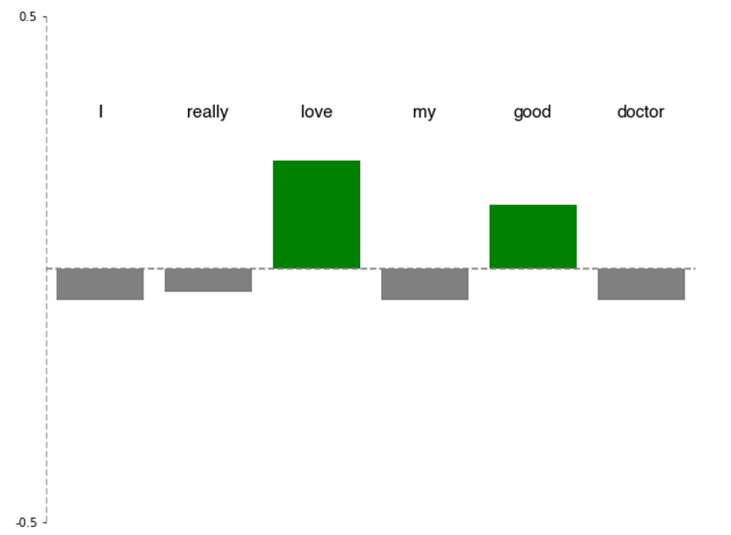
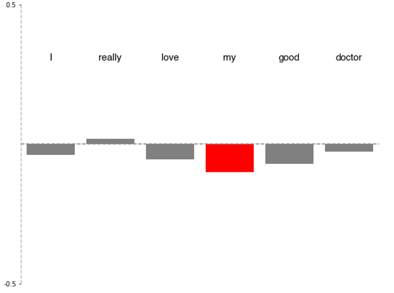
While a poor-performing model may produce word_impact scores like:

We can see from the first example it not only gets the right answer, but also places most of the weight on the important words — “love” and “good”. Noticeably, it does not place much weight on the qualifier “really,” which for this example is not a big deal, but is an important artifact to take note of …even high performing models have artifacts and issues!

The second example performs poorly, and clearly does not know what to look at in the sentence, placing the most emphasis on “my” of all words. While we knew previously this model was bad, we can see that it still is struggling with a fundamental language idea such as adjectives — back to the drawing board!

Conclusion

These are 3 ways to explore bias in your NLP models that my team uses often to explore and iterate before we deploy. These methods are:

1. Using a handcrafted dataset designed to challenge your model and surface potential biases.
2. Analyzing model accuracy across subgroups and verifying the accuracy is comparable for each.
3. Perturbing your inputs to see which words/phrases your model uses to make its prediction.

The right method for you will depend entirely on your model type and the application. The good news is that most common applications and models can leverage a few of these methods.

Hope this was a helpful and informative article! 🚀

Relevant Sources

• https://arxiv.org/pdf/2108.03362.pdf
• https://sethstatistics.files.wordpress.com/2016/08/main.pdf