20 Points to Master Pandas Time Series Analysis

How to handle time series data.

There are many definitions of time series data, all of which indicate the same meaning in a different way. A straightforward definition is that time series data includes data points attached to sequential time stamps.

The sources of time series data are periodic measurements or observations. We observe time series data in many industries. Just to give a few examples:

• Stock prices over time
• Daily, weekly, monthly sales
• Periodic measurements in a process
• Power or gas consumption rates over time

In this post, I will list 20 points that will help you gain a comprehensive understanding of handling time series data with Pandas.

1. Different forms of time series data

Time series data can be in the form of a specific date, time duration, or fixed defined interval.

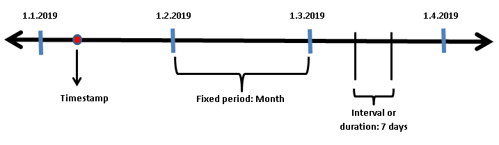
Timestamp can be the date of a day or a nanosecond on a given day depending on the precision. For example, ‘2020–01–01 14:59:30’ is a second-based timestamp.

2. Time series data structures

Pandas provides flexible and efficient data structures to work with all kinds of time series data.

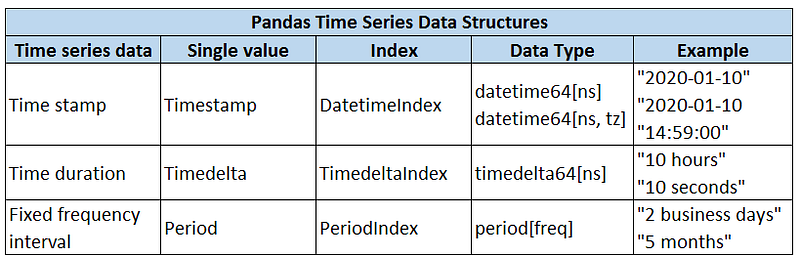
In addition to these 3 structures, Pandas also supports the date offset concept which is a relative time duration that respects calendar arithmetic.

3. Creating a timestamp

The most basic time series data structure is timestamp which can be created using to_datetime or Timestamp functions

import pandas as pd

pd.to_datetime('2020-9-13')
Timestamp('2020-09-13 00:00:00')

pd.Timestamp('2020-9-13')
Timestamp('2020-09-13 00:00:00')

4. Accessing the information hold by a timestamp

We can get information about the day, month, and year stored in a timestamp.

a = pd.Timestamp('2020-9-13')

a.day_name()
'Sunday'

a.month_name()
'September'

a.day
13

a.month
9

a.year
2020

5. Accessing not-so-obvious information

Timestamp objects also hold information about date arithmetic. For instance, we can ask if the year is a leap year. Here are some of the more specific information we can access:

b = pd.Timestamp('2020-9-30')

b.is_month_end
True

b.is_leap_year
True

b.is_quarter_start
False

b.weekofyear
40

6. European style date

We can work with the European style dates (i.e. day comes first) with the to_datetime function. The dayfirst parameter is set as True.

pd.to_datetime('10-9-2020', dayfirst=True)
Timestamp('2020-09-10 00:00:00')

pd.to_datetime('10-9-2020')
Timestamp('2020-10-09 00:00:00')

Note: If the first item is greater than 12, Pandas knows it cannot be a month.

pd.to_datetime('13-9-2020')
Timestamp('2020-09-13 00:00:00')

7. Converting a dataframe to time series data

The to_datetime function can convert a dataframe with appropriate columns to a time series. Consider the following dataframe:

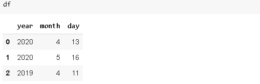
pd.to_datetime(df)

0   2020-04-13 
1   2020-05-16 
2   2019-04-11 
dtype: datetime64[ns]

8. Beyond a timestamp

In real-life cases, we almost always work sequential time series data rather than individual dates. Pandas makes it very simple to work with sequential time series data as well.

We can pass a list of dates to the to_datetime function.

pd.to_datetime(['2020-09-13', '2020-08-12', 
'2020-08-04', '2020-09-05'])

DatetimeIndex(['2020-09-13', '2020-08-12', '2020-08-04', '2020-09-05'], dtype='datetime64[ns]', freq=None)

The returned object is a DatetimeIndex.

There are more practical ways to create sequences of dates.

9. Creating a time series with to_datetime and to_timedelta

A DatetimeIndex can be created by adding a TimedeltaIndex to a timestamp.

pd.to_datetime('10-9-2020') + pd.to_timedelta(np.arange(5), 'D')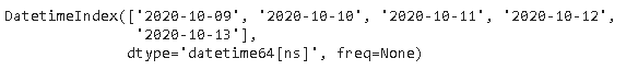

‘D’ is used for ‘day’ but there are many other options available. You can check the whole list here.

10. The date_range function

It provides a more flexible way to create a DatetimeIndex.

pd.date_range(start='2020-01-10', periods=10, freq='M')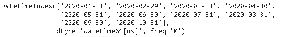

The periods parameter specifies the number of items in the index. The freq is the frequency and ‘M’ indicates the last day of a month.

The date_range is pretty flexible in terms of the arguments for the freq parameter.

pd.date_range(start='2020-01-10', periods=10, freq='6D')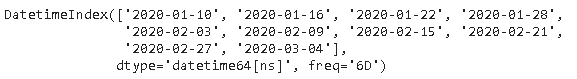

We have created an index with a frequency of 6 days.

11. The period_range function

It returns a PeriodIndex. The syntax is similar to the date_range function.

pd.period_range('2018', periods=10, freq='M')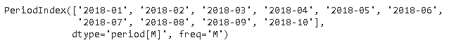

12. The timedelta_range function

It returns a TimedeltaIndex.

pd.timedelta_range(start='0', periods=24, freq='H')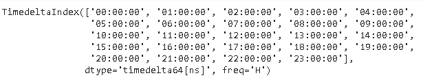

13. Time zones

By default, time series objects of pandas do not have an assigned time zone.

dates = pd.date_range('2019-01-01','2019-01-10')

dates.tz is None
True

We can assign a time zone to these objects using the tz_localize method.

dates_lcz = dates.tz_localize('Europe/Berlin')

dates_lcz.tz
<DstTzInfo 'Europe/Berlin' LMT+0:53:00 STD>

14. Create a time series with an assigned time zone

We can also create a time series object with a time zone using tz keyword argument.

pd.date_range('2020-01-01', periods = 5, freq = 'D', tz='US/Eastern')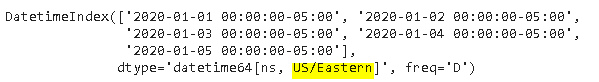

15. Offsets

Consider we have a time series index and want to offset all the dates for a specific time.

A = pd.date_range('2020-01-01', periods=10, freq='D')
A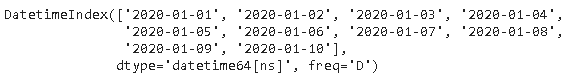

Let’s add an offset of one week to this series.

A + pd.offsets.Week()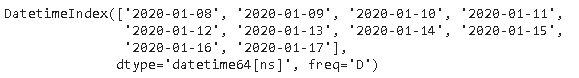

16. Shifting time series data

Time series data analysis may require to shift data points to make a comparison. The shift function shifts data in time.

A.shift(10, freq='M')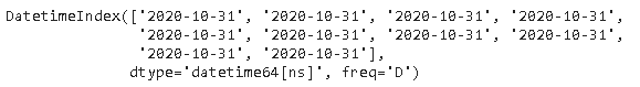

17. Shift vs tshift

• shift: shifts the data
• tshift: shifts the time index

Let’s create a dataframe with a time series index and plot it to see the difference between shift and tshift.

dates = pd.date_range('2020-03-01', periods=30, freq='D')
values = np.random.randint(10, size=30)
df = pd.DataFrame({'values':values}, index=dates)

df.head()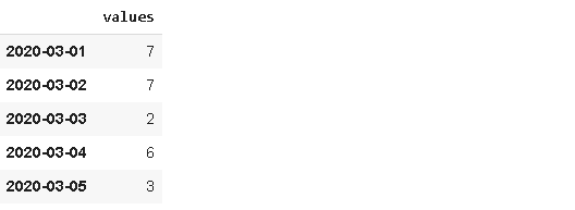

Let’s plot the original time series along with the shifted and tshifted ones.

import matplotlib.pyplot as plt

fig, axs = plt.subplots(nrows=3, figsize=(10,6), sharey=True)
plt.tight_layout(pad=4)
df.plot(ax=axs[0], legend=None)
df.shift(10).plot(ax=axs[1], legend=None)
df.tshift(10).plot(ax=axs[2], legend=None)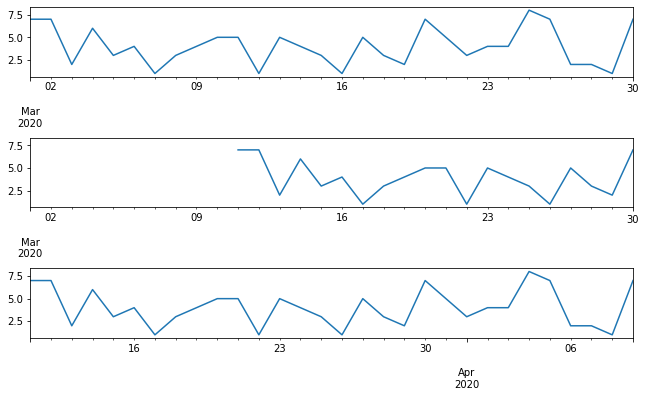

18. Resampling with the resample function

Another common operation with time series data is resampling. Depending on the task, we may need to resample data at a higher or lower frequency.

Resample creates groups (or bins) of specified internal and lets you do aggregations on groups.

Let’s create a Pandas series with 30 values and a time series index.

A = pd.date_range('2020-01-01', periods=30, freq='D')
values = np.random.randint(10, size=30)
S = pd.Series(values, index=A)

The following will return the averages of 3 day periods.

S.resample('3D').mean()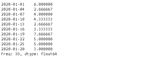

19. Asfreq function

In some cases, we may be interested in the values at certain frequencies. Asfreq function returns the value at the end of the specified interval. For instance, we may only need the values at every 3 days (not a 3-day average) in the series we created in the previous step.

S.asfreq('3D')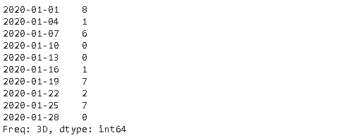

20. Rolling

Rolling is a very useful operation for time series data. Rolling means creating a rolling window with a specified size and perform calculations on the data in this window which, of course, rolls through the data. The figure below explains the concept of rolling.

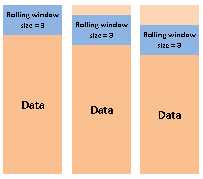
It is worth noting that the calculation starts when the whole window is in the data. In other words, if the size of the window is three, the first aggregation is done in the third row.

Let’s apply a 3-day rolling window to our series.

S.rolling(3).mean()[:10]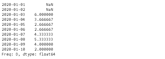

Conclusion

We have covered a comprehensive introduction to time series analysis with Pandas. It is worth noting that Pandas provides much more in terms of time series analysis.

The official documentation covers all the functions and methods of time series. It may seem exhaustive at first glance but you will get comfortable by practicing.

Thank you for reading. Please let me know if you have any feedback.