17 Practice Questions to Learn Pandas’ Data Manipulation and Analysis for a Data Scientist

This post is part of a series of posts where I cover various Data Scientist Role Requirements in Amazon and will cover data manipulation and analysis using Pandas, which is an essential tool for any Data Scientist.

In this post, we will be manipulating a data set from Kaggle, provided by the Guardian. The data set covers the summer Olympic sports and medals spanning from 1896 to 2014 and is named summer.csv.

Next, we will look at the overall topics that will be covered and then will jump to the most fun part, which is the questions and answers. The Jupyter notebook with the questions and answers that you can download and run on your end is provided after the questions and answers.

Now that we know what to expect, let’s get started.

Topics

The following topics will be covered in more detail in this post:

1. Importing and Shape of the Data
2. Series and Data Frames in Pandas
3. Indexing and Slices of the Data
4. Editing Data in a Data Frame
5. Combining Data Frames
6. Grouping and Aggregation

Tutorial + Questions and Answers

I will start with a brief overview of each concept and then most of the learning will be during the practice questions included for each topic. The Jupyter notebook including questions and answers is provided in the next section. To maximize learning, try to answer the questions yourself before looking at the notebook. Then look at the notebook to verify your answers.

1. Importing and Shape of the Data

1.1. Overview

Please start with downloading the data set from here. Once you have the summer.csv downloaded to your local machine, the very first step would be to read the data set into the notebook using Pandas. Since this file is a comma-separated value (CSV), we use pandas.read_csv(). Elsewhere and depending on the format of the file, you may come across others such as:

• pandas.read_excel()
• pandas.read_json()
• pandas.read_html()
• pandas.read_xml()

1.2. Questions

Question 1:

Import summer.csv into a data frame named df and display top 3 rows of the data.

Answer:

import pandas as pd

df = pd.read_csv('summer.csv')
df.head(3)

Results:

We first imported Pandas (if this part is not clear, feel free to refresh the basics that were covered in Python Foundations). Then we get to the importing part of it as follows:

pd.read_csv('file_location/file_name.csv')

This tells Pandas that the file it is about to read is in a csv format and then provides the location of the file. Note that we also need to provide the format extension of the file at the end of the file name as: .csv. In my laptop, I have the data set in the same folder as the Jupyter notebook so I only needed to provide the file_name.csv but it can be in a different folder, which would require adding the file location when you read the file.

Then what happened in df.head(3)?

DataFrame.head(n = 5) is one of the very common functions used to look at the data, which returns the first n rows of the object (i.e. data). If n is not provided, it defaults to 5.

Question 2:

How many rows and columns are in the imported data frame?

Answer:

print(df.shape)

print(f"There are {df.shape[0]} rows and {df.shape[1]} columns in the data frame.")

Results:

What happened?

DataFrame.shape returns a tuple representing the dimensionality of the data frame.

2. Series and Data Frames in Pandas

2.1. Overview

• Series is a one-dimensional data structure in Pandas
• DataFrame is a two-dimensional data structure in Pandas

2.2. Questions

Question 3:

Store the data from column City into a Pandas Series named city.

Answer:

city = df["City"]
type(city)

Results:

Question 4:

How many gold, silver and bronze medals are reported in the data?

Answer:

df["Medal"].value_counts()

Results:

As we saw in this example, Series.value_counts() returns a series containing counts of unique values.

Question 5:

Same as question 4 but instead of count of unique values, return the relative frequencies of the unique values and sort them in an ascending order.

Answer:

df["Medal"].value_counts(normalize = True, ascending = True)

Results:

Question 6:

Find out how many unique country names start with the letter U and how many start with the letter C and save them as u_ct and c_ct, making sure not to count any missing values.

Answer:

# First create a Pandas Series from the 'Country' column and drop the duplicates
country = df["Country"].drop_duplicates()

# Next count how many start with the letters in question
u_ct = country.str.startswith("U", na = False).value_counts()[1]
c_ct = country.str.startswith("C", na = False).value_counts()[1]
print(f"{u_ct} country names start with the letter 'U', while {c_ct} country names start with the letter 'C'.")

Results:

Question 7:

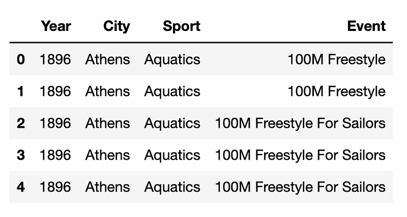
Create a data frame named df_x from the original data frame that only contains the following columns: Year, City, Sport and Event. Then show the top 5 rows of the resulting data frame.

Answer:

df_x = df[['Year', 'City', 'Sport', 'Event']]
df_x.head()

Results:

3. Indexing and Slices of the Data

3.1. Overview

In this part of the exercise, we will try to select specific parts of the data. This is specifically useful since looking at different slices of the data is something that we all do as Data Scientists. In order to do this, we will rely on two new concepts:

• DataFrame.iloc[], which is an integer-location indexing for data selection. In other words, generally when we want to access a group of rows and columns only by referring to their index, we use this iloc[].
• DataFrame.loc[], which access rows and columns by labels. In other words, generally when we want to access a group of rows and columns by their names, we use loc[].

Let’s look at the examples together to better understand the distinction between the two.

3.2. Questions

Question 8:

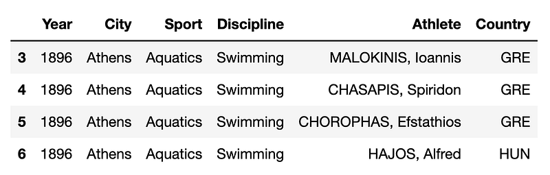
Select rows 3 to 6 (inclusive) and the first 6 columns of the original data frame.

Answer:

df.iloc[3:7, :6]

Results:

Question 9:

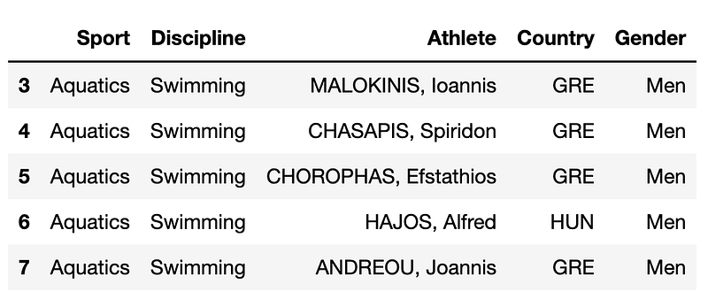
Select rows 3 to 7 (inclusive) and the columns starting from Sport up to and including Gender of the original data frame.

Answer:

df.loc[3:7, "Sport":"Gender"]

Results:

Question 10:

Create a10_1 data frame that includes all the data in the original data frame but only from 1950 and later.

Then create a10_2 data frame that includes all the data in the original data frame but only from the following countries: USA, GBR, FRA and GER.

Finally, verify the results.

Answer:

a10_1 = df.loc[df.Year > 1950]
a10_2 = df.loc[df.Country.isin(["USA", "GBR", "FRA", "GER"])]

print(f"Years in 'a10_1' are: {list(a10_1.Year.unique())}\n")
print(f"Countries in 'a10_2' are: {list(a10_2.Country.unique())}")

Results:

Question 11:

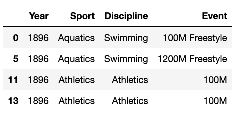
Select rows with index 0, 5, 11, and 13 and the columns with index 0, 2, 3, and 7, from the original data frame and show the results.

Answer:

df.iloc[[0, 5, 11, 13], [0, 2, 3, 7]]

Results:

4. Editing Data in a Data Frame

4.1. Overview

In this section, we will work on changing or deleting some of the values in a data frame.

4.2. Questions

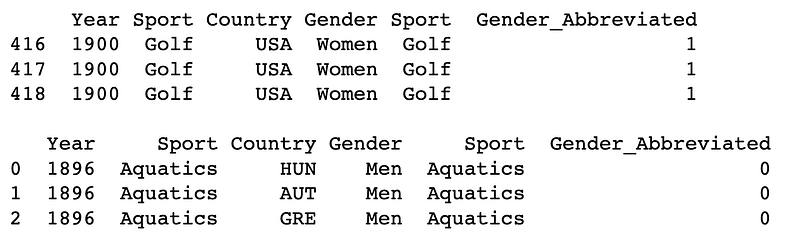
Question 12:

Create the data frame a_12 from the original data frame but only contain the following columns: Year, Sport, Discipline, Country, Gender and Sport.

Then drop the column “Discipline” from a_12.

Then add a new column to a_12 named Gender_Abbreviated that shows 1 for Women and 0 for Men.

Finally, show the first 3 rows of the resulting a_12 for Women and then the same for Men.

Answer:

a_12 = df[['Year', 'Sport', 'Discipline', 'Country', 'Gender', 'Sport']]

a_12 = a_12.drop("Discipline", axis = 1)

a_12["Gender_Abbreviated"] = a_12.Gender.str.contains("W", na = False).astype(int)

print(a_12[a_12["Gender"] == "Women"].head(3))
print("")
print(a_12[a_12["Gender"] == "Men"].head(3))

Results:

5. Combining Data Frames

5.1. Overview

These examples are going to be conceptually similar to Joins and Unions in SQL. Join is when we stick two data sets together next to each other, while Union is when we stack the two data sets on top of each other. Although the SQL knowledge is not a prerequisite here, but if you would like a refresher on these two SQL concepts to follow the analogy, take a look at the SQL Tutorial.

5.2. Questions

Question 13:

Create a data frame named df_y that contains the data in the main data frame from only the following cities: London, Athens, Los Angeles, Beijing, Sydney and Atlanta.

Next, create a new data frame named df_z that includes the cities from df_y and the name of the continent each city is located in. As a refresher, London and Athens are located in Europe, Los Angeles and Atlanta are in North America, Beijing is in Asia, and Sydney is in Oceania.

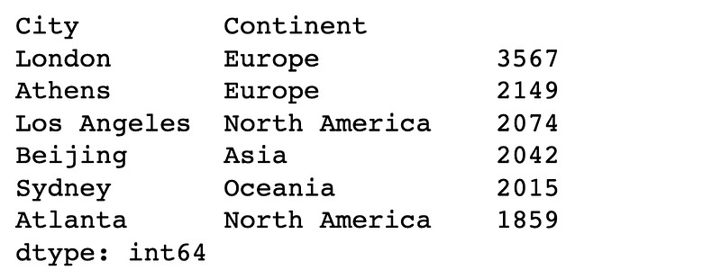
Finally, left join df_y to df_z, using their shared column into df_yz, and then verify that cities are matched correctly to the continents after the join.

Answer:

df_y = df[df['City'].isin(["London", "Athens", "Los Angeles", "Beijing", "Sydney", "Atlanta"])]

df_z = pd.DataFrame(
    {
        'City': ['London', 'Athens', 'Los Angeles', 'Beijing', 'Sydney', 'Atlanta'],
        'Continent' : ['Europe', 'Europe', 'North America', 'Asia', 'Oceania', 'North America']
    }
)

df_yz = pd.merge(df_y, df_z, on = 'City', how = 'left')

df_yz[['City', 'Continent']].value_counts()

Results:

Question 14:

Break the original data frame by half into two separate data frames a14_1 and a14_1 with the same columns (in other words, put half of the rows of df in the first data frame and the remaining rows in the second data frame), verify the resulting shape to make sure there are now two data frames and then stack them back on top of each other to get to the same number of rows of the original data frame.

Answer:

# Number of rows of the original data frame
print(f"df includes {df.shape[0]} rows in total.\n")

# Store the top half into a new data frame and get the number of rows
a14_1 = df.loc[:15582, :]
print(f"a14_1 includes {a14_1.shape[0]} rows.\n")

# Store the bottom half into a new data frame and get the number of rows
a14_2 = df.loc[15583:, :]
print(f"a14_2 includes {a14_2.shape[0]} rows.\n")

# Stack the two halves on top of each other to get the original data frame
a_14 = pd.concat([a14_1, a14_2], ignore_index = True)
print(f"Stacked data frame includes {a_14.shape[0]} rows, compared to the original data frame that had {df.shape[0]} rows.")

Results:

6. Grouping and Aggregation

6.1. Overview

Overarching idea is a simple one — as Data Scientists we are looking for ways to look at aggregated and/or grouped data to be able to extract the underlying information. This section will focus on how to do that in data frames.

6.2. Questions

Question 15:

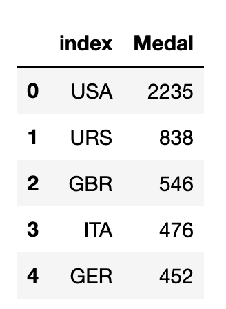
What are the top 5 countries with the highest number of gold medals in total?

Answer:

df[df["Medal"] == "Gold"]["Country"].value_counts().reset_index(name = 'Medal').head()

Results:

Question 16:

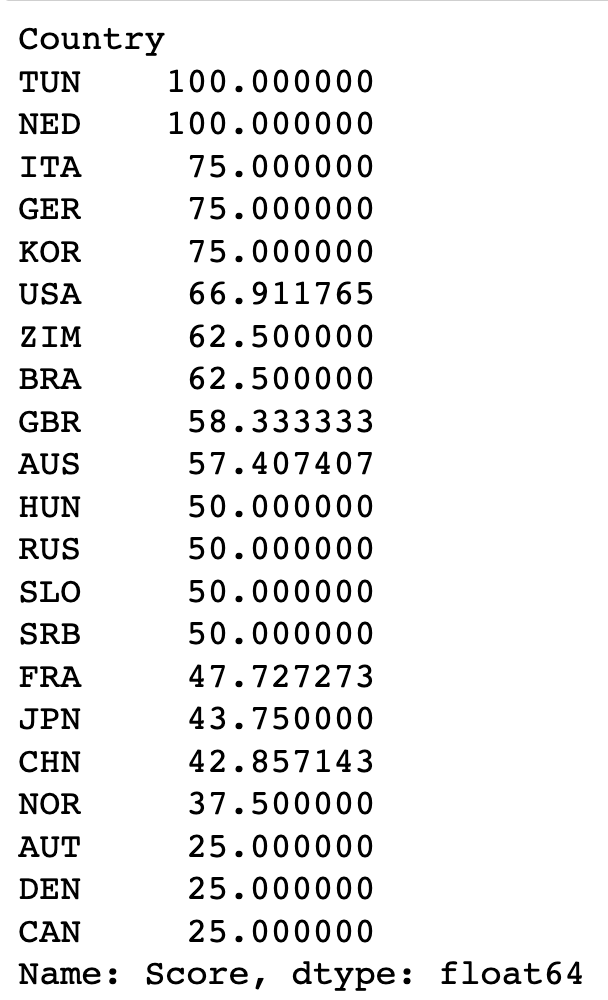
Create a new column in the original data frame named Score according to each medal. For the purposes of this exercise, gold is worth 100, silver is 50, while bronze is worth 25 points. Then find the average of points by country in 2008 Olympics in the swimming discipline and sort the results in a descending order.

Note: We could use pd.DataFrame.merge() for this exercise, similar to question 13 but we will be exploring an alternative approach here for learning purposes.

Answer:

# Duplicate the Medal column
df['Score'] = df.loc[:, 'Medal']

# Replace each medal with its score
df = df.replace({'Score': {'Gold':100, 'Silver': 50, 'Bronze': 25}})

# Filter and group by
df[(df["Year"] == 2008) & (df["Discipline"] == "Swimming")].groupby("Country")["Score"].mean().sort_values(ascending = False)

Results:

Question 17:

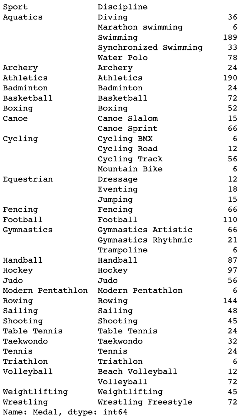
Some sports include more than one disciplines. How many total medals were given in Olympics 2012 for each sport and discipline?

Answer:

df[(df["Year"] == 2012)].groupby(["Sport", "Discipline"])["Medal"].count()

Results:

Notebook

Below is the notebook with both questions and answers for reference.

Thanks for Reading!

If you found this post helpful, please follow me on Medium and subscribe to receive my latest posts!