Classification Intro & Implementation — Logistic Regression vs. K-Nearest Neighbors vs. Naive Bayes

We continue learning about the Technical Requirements to Become a Data Scientist, by expanding into classification. We are going to look at a classification task and implement Logistic Regression, K-Nearest Neighbors and Naive Bayes and compare their performance in predicting the outcome.

Steps we will take in this post are as follows:

1. Data Preparation: This will include familiarizing ourselves with the data, labeling the target variable, feature selection and scaling, dummy coding and some clean-up (e.g. dealing with null values)
2. Model Evaluation: In this part and before getting to the modeling part, we will first go over some of the most common evaluation metrics/presentations in classification tasks, such as accuracy, precision, recall and confusion matrix
3. Model Selection: Then we will learn more about each of the classifiers, including Logistic Regression, K-Nearest Neighbors and Naive Bayes, build models using each of them and then compare their performance, using the evaluation methodologies we learned in the previous step.

As usual, learning happens with the help of the questions and as we go through these questions together. I will include tips and explanation for each question to make the journey easier. Lastly, the notebook that I used for this exercise is also linked in the bottom of the post, which you can download, run and follow along.

Let’s get started!

1. Data Preparation

1.1. Data Overview

We will be using a dataset from Kaggle that is based on the U.S. Department of Transportation’s Bureau of Transportation Statistics, tracking on-time performance of domestic flights in year 2008. The dataset can also be downloaded from this link. Note that the original file is quite large so I filtered it only to flights to and from JFK airport in NYC.

Column names are generally self-explanatory. Let’s familiarize ourselves with the data by looking at a few rows.

# Import libraries
import pandas as pd
import numpy as np

# To show all the columns
pd.set_option("display.max_columns", None)

# To show all columns in one view
from IPython.display import display, HTML
display(HTML("<style>.container { width:100% !important; }</style>"))

Now let’s read the data and display the top 5 rows.

df = pd.read_csv('DelayedFlights_JFK.csv')
df.head()

Looking at the data above, it looks like the very first column did not have a column name and therefore Pandas has assigned Unnamed: 0 to it. This does not cause a problem but we can also prevent this from happening. One solution is to instruct Pandas to use that very first column as the index for the dataframe, as shown below:

df = pd.read_csv('DelayedFlights_JFK.csv', index_col=[0])
df.head()

Now the Unnamed: 0 column is gone and its values are being used as the index of the dataframe. Let’s see how many rows and columns are there in the data.

df.shape

Our dataframe consists of 70,212 rows and 29 columns so far. This might be helpful to keep in mind in case we decide to drop any of the rows or columns in the future.

1.2. Data Preparation — Labeling

Question 1:

We plan to create a model to predict whether a flight will be delayed or not but there are also some rows that indicate cancelled flights in our dataframe. Let’s just delete the rows where a flight was cancelled (use column Cancelled).

Answer:

Let’s first find out how many flights were cancelled.

df.Cancelled.value_counts()

Results:

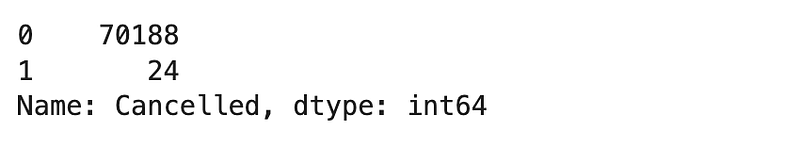
24 flights were cancelled (which I personally find surprisingly low…) but let’s continue.

Now let’s go ahead and drop these 24 entries (where df[Cancelled] == 1) from our dataframe.

df.drop(df[df['Cancelled'] == 1].index, inplace = True)

Let’s make sure the changes are as we expected.

df.Cancelled.value_counts()

Results:

Now we see that we no longer have any rows with a cancelled flight.

Question 2:

Create a new column named delayed. If a flight is delayed longer than 15 minutes, it should be considered delayed and labeled as 1. If delayed less than or equal to 15 minutes, it is not considered delayed and can be marked as 0. Column ArrDelay shows the arrival delay in minutes.

Fun Fact: I was curious about how much delay is actually considered a delayed flight and according to Wikipedia, U.S. Federal Aviation Administration (FAA) considers a flight to be delayed when it is 15 minutes later than its scheduled time.

Answer:

df['delay'] = [1 if x > 15 else 0 for x in df['ArrDelay']]

Let’s look at our newly created column to see how balanced these two classes are (i.e. we want to look at delayed, indicated by 1, and not-delayed, indicated by 0, and see what ratio of the total data they each account for).

df['delay'].value_counts(normalize = True)

Results:

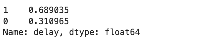
Based on this data and above definition of a delayed flight, almost 69% of flights to and from JFK were delayed, while the remaining 31% were not. I find this more aligned with my personal experience of flying to/from JFK, especially in the past few years.

1.3. Data Preparation — Feature Selection

At this point of the exercise, we would like to focus on determining what columns to use as features (or independent variables) for the task of classification. We will start by looking at columns that may seem duplicative and would not provide new information.

Question 3:

Take a look at the columns, identify which ones may provide the same information and drop them.

Answer:

Let’s look at the columns first.

df.columns

Results:

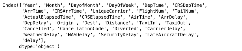
Below are the columns that I think can be dropped. Go through this and feel free to make changes to this list based on your judgement.

- Year: We know all flights are in the same year of 2008. - FlightNum: Flight number is an arbitrary value. - CancellationCode: We excluded cancelled flights from our data so this one does not offer any predictive value.

Let’s drop these columns.

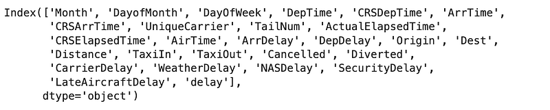
df.drop(['Year', 'FlightNum', 'CancellationCode'], axis = 1, inplace = True)

And let’s double check our changes. Feel free to experiment with dropping additional columns and you can see the impact on predictive power later on in the exercise.

df.columns

Results:

1.4. Data Preparation — Dummy Coding

Question 4:

Create a new column named jfk_origin, which will take a value of 1 when the origin is JFK and otherwise takes a 0 (i.e. this indicates JFK was the destination airpot, since we have limited the dataframe to only to and from JFK). Then take a look at the weight of each of these two classes in thew newly-created column.

Answer:

Let’s first create the new column.

df['jfk_origin'] = [1 if x == 'JFK' else 0 for x in df['Origin']]

Now let’s look at the weight of each of the classes in this newly-created column.

df['jfk_origin'].value_counts(normalize = True)

Results:

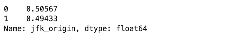
The jfk_origin column seems almost perfectly balanced, as expected. In other words, almost half of the flights are to and the other half are from JFK, which intuitively makes sense.

1.5. Data Preparation — Additional Clean-Up

1.5.1. Additional Clean-Up — Drop Unnecessary Columns

Next we want to take out some additional columns from the data set, to further cleanup the data. Below are the columns that I am going to take out, along with the reasons. Feel free to remove additional or fewer columns and investigate the impact on the model performance.

• Origin: There are way too many origins to dummy code and we have our new jfk_origin column to work with.
• Dest: There are way too many origins to dummy code and we have our new jfk_origin column to work with.
• ArrDelay: Arrival delay will be known only after a delayed arrival so it is not a data point that would be available to us to predict whether a flight will be delayed.
• DepDelay: Departure delay is what will be known only after a delayed departure so it is not a data point that would be available to us to predict whether a flight will be delayed.
• UniqueCarrier: Indicates airline’s unique identifyer. Dropping because there are too many to dummy code.
• TailNum: Unique aircraft identification number. Dropping because there are too many to dummy code.
• CarrierDelay: This is a type of a delay, which we would not know until after the delay has happened so we cannot use this in our predictions.
• WeatherDelay: This is a type of a delay, which we would not know until after the delay has happened so we cannot use this in our predictions.
• NASDelay: This is a type of a delay, which we would not know until after the delay has happened so we cannot use this in our predictions.
• SecurityDelay: This is a type of a delay, which we would not know until after the delay has happened so we cannot use this in our predictions.
• LateAircraftDelay: This is a type of a delay, which we would not know until after the delay has happened so we cannot use this in our predictions.

So let’s go ahead and drop these columns.

df.drop(['Origin', 'Dest', 'ArrDelay', 'DepDelay', 'UniqueCarrier', 'TailNum', 'CarrierDelay', 'WeatherDelay', 'NASDelay', 'SecurityDelay', 'LateAircraftDelay'], axis = 1, inplace = True)

1.5.2. Additional Clean-Up — Null Values

Now that we have taken out some columns, let’s also look at the null values or Not-a-Numbers (NANs). There are different strategies when dealing with NANs. For example, sometimes based on the business knowledge or deeper familiarity with the datat, we can decide to replace NANs with certain values. In this case we will most likely just drop the rows where such NANs exist in our data.

Let’s look at the number of NANs and what columns they are in.

df.isnull().sum()

Results:

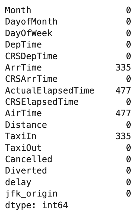
There does not seem to be that many rows so we can go ahead and drop those. We will also look at how many rows exist before and after this step for our information.

print(f"There are {df.shape[0]} rows before taking out null values.\n")

# Drop rows with null values in them
df = df.dropna()

print(f"There are {df.shape[0]} rows after taking out null values.")

Results:

We can see the difference between the two values and we still have 69,711 rows in the dataframe.

1.6. Data Preparation — Splitting the Data into Train and Test Sets

Question 5:

Break down the data into predictors (X or independent variables) and target variable (y or dependent variable).

Answer:

X = df.drop(['delay'], axis = 1)
y = df['delay']

Question 6:

Split the data into train (70%) and test (30%) sets, using a random_state of 1234.

Hint: Use train_test_split from sklearn.model_selection.

Answer:

from sklearn.model_selection import train_test_split

X_train, X_test, y_train, y_test = train_test_split(X, y, test_size = 0.3, random_state = 1234)

1.7. Data Preparation — Feature Scaling

An important part of data pre-processing is feature scaling, which ensures the training data is in the same scale. More formally, feature scaling normalizes the range of independent variables (or features). This is sometimes referred to as normalization.

Feature sclaing ensures the objective function of the machine learning algorithms work properly. For example, some classifiers use the Euclidean distance between two points. Euclidean distance between two points is the length of the line that connects those two points. If one of the features has a broad range of values (compared to others), it will overpower all other distances. To make this “normal”, we normalize the scale of all features using a feature scaling methodology.

In our specific example, Logistic Regression and K-Nearest Neighbors use the magnitude of distance between points among features. This means that if the values of one of our features/columns have large variations, such as DepTime and ArrTime, compared to DayOfWeek, then those columns will have a different weight in the model.

The good news is that sklearn.preprocessing.StandardScaler() does this for us so we will use that in the next question.

Question 7:

Apply feature scaling to our train and test features (i.e. X_train and X_test).

Answer:

# Import packages
from sklearn.preprocessing import StandardScaler

sts = StandardScaler()
X_train = sts.fit_transform(X_train)
X_test = sts.transform(X_test)

2. Model Evaluation

Before we start with the model selection process, we are going to cover a few evaluation metrics that are normally used in classification tasks.

2.1. Model Evaluation — Accuracy

In a two-class target variable where the target variable can only be positive (or 1) and negative (or 0), there are four possible outcomes for a prediction:

1. True Positive (TP): A positive event was correctly predicted.
2. False Positive (FP): A negative event was incorrectly predicted as positive. This is also known as a Type I error.
3. True Negative (TN): A negative event was correctly predicted.
4. False Negative (FN): A positive event was incorrectly predicted as negative. This is also known as a Type II error.

Accuracy is the proportion of correct predictions over total predictions. Using the outcomes described above, we can create an equation for Accuracy as follows:

2.2. Model Evaluation — Confusion Matrix

Confusion matrix is a tabular presentation of the results of a classification exercise. We looked at Accuracy previously, which calculates the proportion of correct predictions out of total predictions. But it does not report on what percentage of predictions were incorrectly predicted. This shortcoming is more apparent in scenarios with more than 2 classes and also where the data is imbalanced. For example, if we had 3 classes of A, B and C that each accounted for 80%, 15% and 5% of total and then accuracy of the model is 80%, what does that mean? There is a possibility that our model is really not doing anything and for any entry, it is just returning A. Then all of predictions are A but we are still getting 80% accuracy because A accounted for 80% of the total data. Confusion matrix helps by adding more context in such scenarios.

Let’s create a table to show these four outcomes:

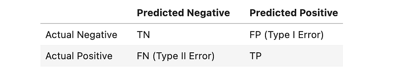
This tabular presentation is called a confusion matrix. More formally, a confusion matrix C is such that C(i,j) is equal to the number of observations known to be in group i and predicted to be in group j. Therefore, in a binary classification, the count of true negatives is C(0,0), false negatives is C(1,0, true positive is C(1,1), and false positives is C(0,1).

Note: Placement of TP, FP, TN, and FN in a confusion matrix is simply based on an agreement. In other words, they can move around, based on how the confusion matrix is defined. In this exercise, I have used the placement that sklearn.metrics.confusion_matrix uses, since we will be using that later on in the exercise.

2.3. Model Evaluation — Precision and Recall

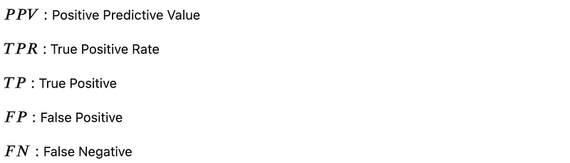
Precision and Recall are two of the performance metrics that you will hear about in the context of classification. Precision, also called Positive Predictive Value (PPV), is the fraction of relevant instances among the retrieved instances, while Recall, also called Sensitivity or True Positive Rate (TPR), is the fraction of relevant instances that were retrieved. Let’s use the terminology that we have learned so far and convert the textual definitions to equations to better understand these two:

Precision and recall can be calculated by precision_score and recall_score from sklearn.metrics, respectively.

These concepts will become easier to understand as we go through the exercises, so let’s dive into the modeling part.

3. Model Selection

At this point, the data is ready and it is time for us to proceed with our model selection. We will be experimenting with three classification models:

1. Logistic Regression
2. K-Nearest Neighbors
3. Naive Bayes

For each one, we will go over a brief overview, then will train the model, followed by evaluating the performance of the model. Finally we can compare the evaluation results and decide which model works best for our experiment.

3.1. Model Selection — Logistic Regression

Logistic Regression, despite its name, is a classification algorithm where the dependent variable can only take two classes (e.g. yes vs. no or 0 vs. 1). Classification problems with only two possible outcomes for the dependent variables are called binary classifications.

Logistic regression relies on the logistic function, which is a Sigmoid curve with the following equation:

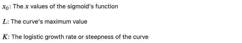
If we assume L = 1, k = 1, and x0 = 0, then the curve will look as follows:

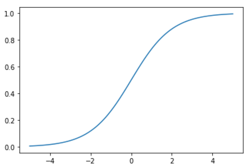
A logistic regression model calculates the probability based on the formula above, which will always end up between 0 and 1. Then when the probability is between 0 and 0.5 (assuming a 50% threshold), assigns it to one class, such as 0 or not-spam and then when the probability is between 0.5 and 1, assigns it to the other outcome, such as 1 or spam.

Question 8:

Use logistic regression to train a model on the training data, then create predictions for the test set and name them as y_pred_lr. For consistency, use a random_state of 1234 and a solver of lbfgs.

Hint: We can use LogisticRegression from sklearn.linear_model.

Notes:

• solver: We used the lbfgs solver here, which is the default solver for this model and is a good one for multiclass problems. Other solves are also available and can be used based on the type of the problem, for example, liblinear is usually a good choice for small datasets since it is not very fast. On the other hand, we might have used sag or saga for larger datasets, since those are faster.
• Documentation: Further details can be found here.

Answer:

# Import LogisticRegression
from sklearn.linear_model import LogisticRegression

# Train the model
lr = LogisticRegression(random_state = 1234, solver = 'lbfgs')
lr.fit(X_train, y_train)

# Predict the test set
y_pred_lr = lr.predict(X_test)

Question 9:

Create the confusion matrix for the logistic regression model on the test set and then calculate the accuracy to measure the performance of the classifier.

Hint: We can use confusion_matrix from sklearn.metrics to generate the confusion matrix. sklearn.linear_model.LogisticRegression.score() can be used to calculate accuracy.

Answer:

# Import confusion matrix
from sklearn.metrics import confusion_matrix

# Create the confusion matrix
cm_lr = confusion_matrix(y_test, y_pred_lr)
print("Logistic Regression's Confusion Matrix:")
print(f"{cm_lr}\n")

# Calculate accuracy score
lr_score = lr.score(X_test, y_test)
print("Logistic Regression's Accuracy:")
print(lr_score)

Results:

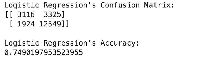
Our logistic regression model has an accuracy of around 74.9%. Let’s keep that number in mind for comparison as we move to test other classifiers.

3.2. Model Selection — K-Nearest Neighbors

K-Nearest Neighbors or KNN is a supervised learning method where an object is classified by a plurality vote of its neighbors. What it means is that the object will be assigned a class that is most common among its k nearest neighbors (based on distance).

KNN is easy to set up using the neighbors.KNeighborsClassifier(n_neighbors = 5, p = 2) from sklearn. n_neighbors is the number of neighbors to use, which is 5 by default. p is the power parameter for the Minkowski metric. When p = 1, it is equivalent to using Manhattan distance or L1 (which is a distance metric between two points in a N-dimensional vector space). When p = 2, it just uses Euclidean distance or L2 (which is the lenght of a line between two points and is usually how we normally think about distance in real life).

This level of knowledge will suffice for our use case but in case you are curious to learn more, you can take a look at the documentation.

Now that we are more familiar with KNN, let’s look at an example.

Question 10:

Use KNN to train a model on the training data, then create predictions for the test set and name them as y_pred_knn. For the sake of consistency, use n_neighbors = 10 and use the Manhattan distance (i.e. p = 1).

Answer:

# Import KNN
from sklearn.neighbors import KNeighborsClassifier

# Train the classifier
knn = KNeighborsClassifier(n_neighbors = 10, p = 1)
knn.fit(X_train, y_train)

# Crate predictions
y_pred_knn = knn.predict(X_test)

Question 11:

Create the confusion matrix for the KNN model on the test set and then calculate the accuracy to measure the performance of the classifier.

Answer:

# Create the confusion matrix
cm_knn = confusion_matrix(y_test, y_pred_knn)
print("KNN's Confusion Matrix:")
print(f"{cm_knn}\n")

# Calculate accuracy score
knn_score = knn.score(X_test, y_test)
print("KNN's Accuracy:")
print(knn_score)

Results:

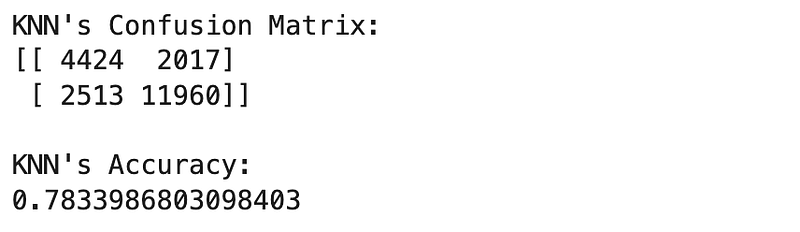
It looks like we improved a bit. Accuracy moved from around 75% in Logistic Regression to over 78% in KNN.

Let’s move on to the next classifier and see if that can improve our classification results.

3.3. Model Selection — Naive Bayes

Naive Bayes calculates the probability of a data point belonging to a certain class. It is called Naive because it assumes the occurrence of a certain feature is independent of the occurrence of other features. And it is called Bayes since it relies on Bayes’ Theorem, described below. For the purposes of this exercise, you can just remember that Naive Bayes is a type of classification model and do not need to understand the Bayes’ Theorem.

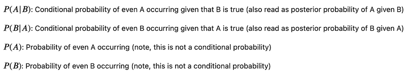
One of the assumptions of this model is that features are independent, which might not be the case in our example and we would not expect a good performing model but the goal here is to learn how to use this classifier so let’s move forward.

For our modeling purposes, we can use the naive_bayes.GaussianNB() class from sklearn. If you are interested to learn more about it, you can look at the documentation here but this level of knowledge is enough for us to move on at this point.

Question 12:

Use Naive Bayes to train a model on the training data, then create predictions for the test set and name them as y_pred_nb.

Answer:

# Import Naive Bayes
from sklearn.naive_bayes import GaussianNB

# Train the classifier
nb = GaussianNB()
nb.fit(X_train, y_train)

# Create the predictions
y_pred_nb = nb.predict(X_test)

Question 13:

Create the confusion matrix for the Naive Bayes model on the test set and then calculate the accuracy to measure the performance of the classifier.

Answer:

# Create the confusion matrix
cm_nb = confusion_matrix(y_test, y_pred_nb)
print("Naive Bayes' Confusion Matrix:")
print(f"{cm_nb}\n")

# Calculate accuracy score
nb_score = nb.score(X_test, y_test)
print("Naive Bayes' Accuracy:")
print(nb_score)

Results:

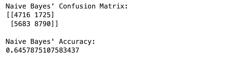
As we suspected, the accuracy is lower than both Logisitc Regression and KNN. But accuracy is not the only metric we should consider for in model evaluation. Let’s also look at Precision and Recall.

Question 14:

Calculate accuracy, precision and recall for all three classifiers and make a decision on the best performing model among the three.

Answer:

# Import required classes
from sklearn.metrics import precision_score, recall_score

# Precision and recall for Logisitc Regression
lr_precision = precision_score(y_test, y_pred_lr)
lr_recall = recall_score(y_test, y_pred_lr)

# Precision and recall for KNN
knn_precision = precision_score(y_test, y_pred_knn)
knn_recall = recall_score(y_test, y_pred_knn)

# Precision and recall for Naive Bayes
nb_precision = precision_score(y_test, y_pred_nb)
nb_recall = recall_score(y_test, y_pred_nb)

# Print the results for comparison
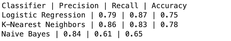
print("Classifier | Precision | Recall | Accuracy")
print(f"Logistic Regression | {round(lr_precision, 2)} | {round(lr_recall, 2)} | {round(lr_score, 2)}")
print(f"K-Nearest Neighbors | {round(knn_precision, 2)} | {round(knn_recall, 2)} | {round(knn_score, 2)}")
print(f"Naive Bayes | {round(nb_precision, 2)} | {round(nb_recall, 2)} | {round(nb_score, 2)}")

Results:

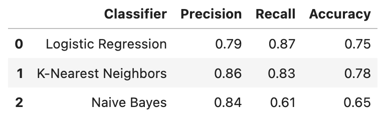
If you want the results to be more presentable, you can also save them as a dataframe, as follows:

# Place the results in a dictionary, which we will use to create a dataframe from
results = {'Classifier':['Logistic Regression', 'K-Nearest Neighbors', 'Naive Bayes']
           , 'Precision': [round(lr_precision, 2), round(knn_precision, 2), round(nb_precision, 2)]
           , 'Recall': [round(lr_recall, 2), round(knn_recall, 2), round(nb_recall, 2)]
           , 'Accuracy': [round(lr_score, 2), round(knn_score, 2), round(nb_score, 2)]
          }

# Create the results dataframe from the results dictionary
df_r = pd.DataFrame(results)
df_r

Results:

But how can we decide which model is the “best” one among the three? This is a harder question to answer than it sounds. If we are looking for a higher precision (i.e. we are more concenred about false positives, according to the equation of calculating precision), then KNN is the way to go but if we care more about recall (i.e. we are more concerend about false negatives), then Logistic Regression is a better classifier.

Conclusion

In this post we implemented three common classification models, Logistic Regression, K-Nearest Neighbors and Naive Bayes. Then we leveraged various evaluation metrics and methodologies, such as Accuracy, Precision, Recall and Confusion Matrix to decide what models suits our needs. As expected, each classifier has its own unique advantages and disadvantages. For example, Logistic Regression provided the highest Recall among the three classifiers, while K-Nearest Neighbors demonstrated the highest Precision and Accuracy. We also implemented Naive Bayes, which does not seem to be a preferred choice for this problem.

The final conclusion is that each problem and task is unique and depending on such specific requirements, we will make a decision on what models to use.

Notebook with Practice Questions

Below is the notebook with both questions and answers that you can download and practice.

Thanks for Reading!

If you found this post helpful, please follow me on Medium and subscribe to receive my latest posts!