
10 quick Numpy tricks that will make life easier for a data scientist
Learn essential Numpy functions for data science

Numpy was the only thing that made me, a die-hard C++ coder, shift to python in the first place. Mind you, this was before my data science learning curve, where no one can survive without python! (No offense, please, just stating my opinion, all the R lovers, I respect you guys all the same). But if one library can change my loyalty to a programing language, then it must be one hell of a library.
In the robotics lab that I interned at once, we used to quiz each other on weird Numpy commands, and that is when I got to see the beauty of this library truly. So if you pass the following test, by all means, you don’t need this blog :P. But otherwise, keep reading!!
Test: Predict the output of the following
import numpy as nparr = np.arange(5)
arr = arr[-1::-1]
print(arr)If you already know this, you probably know most of what I will cover through this blog but otherwise, keep reading.
Output is [4,3,2,1,0]
Let’s dive into functions of Numpy that make it a lifesaver for us, especially for me because I hate writing double for loops to access a 2D array.
Note: In all future examples, I have assumed that import numpy as np has been called
1. numpy.arange(start, stop, step)
This function returns a numpy array that contains numbers starting from start ending before stop and increasing with a difference of step. So the numbers lie in [start, stop) interval.
For example,
>>> np.arange(3,7,2)
array([3, 5])
>>> np.arange(5)
array([0,1,2,3,4])Similar functions: numpy.linspace, numpy.repeat, numpy.tile, numpy.eye(it's a different use case but helpful when dealing with matrices).
If you want to see other ways to define and initialize an array, I have mentioned them in my previous blog here.
2. numpy.random
numpy.random is a module in NumPy that contains functions used for generating random numbers. It can be used for several purposes and is especially important when we deal with probability-based functions. Let’s look at a couple of examples of different functions from this module. The outputs shown below will change when you use the same commands since they are randomly generated.
#Create an array of random numbers, size of array is (3,2)>>> np.random.rand(3,2)
array([[ 0.14022471, 0.96360618], #random
[ 0.37601032, 0.25528411], #random
[ 0.49313049, 0.94909878]]) #randomCheck out more examples here.
#Return random integers from low (inclusive) to high (exclusive) or 0 (inclusive) to low(exclusive), random.randint(low, high=None, size=None, dtype=int)>>> np.random.randint(2, size=10)
array([1, 0, 0, 0, 1, 1, 0, 0, 1, 0]) # random
>>> np.random.randint(5)
1Check out more examples here.
Similar functions: numpy.random.randn, numpy.random.random_sample, numpy.random.choice.
3. numpy.argmax(arr, axis = None)
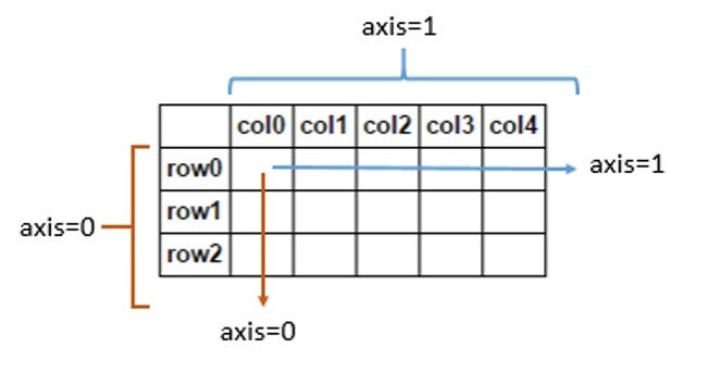
A lot of our use cases, especially when performing optimization, require us to know the variable that has the maximum or minimum value. To get rid of the extra lines of code to keep track of this information, we can simply use the numpy functions of argmax and argmin. Let’s see an example of the same. The following examples contain the term axis. Axis for an array is the direction along which we want to perform the calculations. If we don’t specify an axis, then the calculations are done over the complete array by default.
>>> a = np.array([[10, 12, 11],[13, 14, 10]])
>>> np.argmax(a)
4 #since if the array is flattened, 14 is at the 4th index
>>> np.argmax(a, axis=0)
array([1, 1, 0]) # index of max in each column
>>> np.argmax(a, axis=1)
array([1, 1]) # index of max in each row
Similar functions: numpy.argmin, numpy.amax
4. Slicing and Indexing
This plays a crucial role in changing the content of a NumPy array. It is used to access multiple elements of an array at the same time. Taking an example would make it easier for you to understand how it works.
>>> a = np.arange(5)
>>> print(a[4])
4 # number at index
>>> print(a[1:])
array([1, 2, 3, 4]) #it will print all element from index 1 to last (including number at index 1)>>> print(a[:2])
array([0, 1]) #it will print all element from index 0 to index 2(excluding number at index 2)>>> print(a[1:3])
array([1, 2]) #it will print all element from index 1 (including) to index 3 (excluding)>>> print(a[0:4:2])
array([0,2]) # [0:4:2] represents start index, stop index, and step respectively. It will start from index 0 (inclusive) go to index 4 (exclusive) in step of 2 which will result in [0, 2] and a[0,2] will be the output.Slicing is used to access elements at multiple indexes of a numpy array smartly. If used properly, it could reduce the length of code by a drastic amount.
Jumping back to the test I gave at the beginning of the blog, the sorcery there was using slicing. When we wrote arr[-1::-1] it essentially started at the last element of arr and then the second -1 ensured that it went in reverse order with step size 1. Hence we got the reverse array.
5. numpy.setdiff1d(ar1, ar2)
When we need to treat our arrays as sets and find their difference, intersection or union, numpy makes the job easy by these inbuilt functions.
#Set difference
>>> a = np.array([1, 2, 3, 2, 4, 1])
>>> b = np.array([3, 4, 5, 6])
>>> np.setdiff1d(a, b)
array([1, 2])
#Set intersection
>>> np.intersect1d([1, 3, 4, 3], [3, 1, 2, 1])
array([1, 3])#Set Union
>>> np.union1d([-1, 0, 1], [-2, 0, 2])
array([-2, -1, 0, 1, 2])Similar functions: numpy.setxor1d, numpy.isin.
6. numpy.reshape(a, newshape, order=’C’)
When dealing with matrices, we need proper dimensions when multiplying and such. Or even when dealing with complex data, I have had to change the shape of my arrays countless times.
>>> a = np.arange(6).reshape((3, 2))
>>> a
array([[0, 1],
       [2, 3],
       [4, 5]])
>>> np.reshape(a, (2, 3)) # C-like index ordering
array([[0, 1, 2],
       [3, 4, 5]])
>>> np.reshape(a, (2, 3), order='F') # Fortran-like index ordering
array([[0, 4, 3],
       [2, 1, 5]])
Check out more examples here. ( I strongly recommend reading all the examples)
Similar functions: ndarray.flatten, numpy.ravel. Both of these changes any array into a 1D array, but there are subtle differences between the two. Also, functions like numpy.squeeze, and numpy.unsqueeze are used to remove or add one dimension in the array.
7. numpy.where(condition[, x, y])
np.where helps us extract a subarray with respect to some condition that we input to the function. Here if the condition is satisfied, then x is chosen or else y. Let’s see some examples to understand more
>>> np.where([[True, False], [True, True]],
...          [[1, 2], [3, 4]], #x
...          [[9, 8], [7, 6]]) #y
#Here since the second element in first row was false the output contained the element from the second array at that index.
>>> a = np.arange(10)
>>> a
array([0, 1, 2, 3, 4, 5, 6, 7, 8, 9])
>>> np.where(a < 5, a, 10*a)
array([ 0, 1, 2, 3, 4, 50, 60, 70, 80, 90])Similar functions: np.choose, np.nonzero
8. numpy.concatenate((a1, a2, …), axis=0)
This function helps join arrays along an existing axis. It is beneficial when we preprocess data and need to append or combine it multiple times.
>>> a = np.array([[1, 2], [3, 4]])
>>> b = np.array([[5, 6]])
>>> np.concatenate((a, b), axis=0)
array([[1, 2],
       [3, 4],
       [5, 6]])
>>> np.concatenate((a, b.T), axis=1)
array([[1, 2, 5],
       [3, 4, 6]])
>>> np.concatenate((a, b), axis=None)
array([1, 2, 3, 4, 5, 6])
Similar functions: numpy.array_split, numpy.ma.concatenate, numpy.split, numpy.hsplit, numpy.vsplit, numpy.dsplit, numpy.hstack
9. numpy.power(x1, x2)
I can’t tell you how much this function has made my life easier truly. It has helped me replace all the loops I used to write to square or cube a whole array. This function outputs an array that contains the first array’s elements raised to powers from the second array, element-wise. Let me show you an example to make things clear.
>>> x1 = np.arange(6)
>>> x1
[0, 1, 2, 3, 4, 5]
>>> np.power(x1, 3)
array([  0,   1,   8,  27,  64, 125])
>>> x2 = [1.0, 2.0, 3.0, 3.0, 2.0, 1.0]
>>> np.power(x1, x2)
array([  0.,   1.,   8.,  27.,  16.,   5.])
>>> x2 = np.array([[1, 2, 3, 3, 2, 1], [1, 2, 3, 3, 2, 1]])
>>> x2
array([[1, 2, 3, 3, 2, 1],
       [1, 2, 3, 3, 2, 1]])
>>> np.power(x1, x2)
array([[ 0,  1,  8, 27, 16,  5],
       [ 0,  1,  8, 27, 16,  5]])
The ** operator can be used as a shorthand for np.power on ndarrays.
Similar functions: All the basic mathematical operators. You can check them out here.
10. numpy.allclose(a, b,rtol=1e-5, atol=1e-8)
np.allclose is used to determine if two arrays are element-wise equal within a tolerance. The tolerance value is positive and a small number. It is calculated as the sum of (rtol * abs(b)) and atol. The element-wise absolute difference between a and b should be less than the calculated tolerance.
>>> np.allclose([1e10,1e-7], [1.00001e10,1e-8])
False
>>> np.allclose([1e10,1e-8], [1.00001e10,1e-9])
True
This proves extremely helpful when comparing two arrays containing prediction values from two different models.
Similar functions: numpy.isclose, numpy.all, numpy.any, numpy.equal
I gladly certify you as the Numpy master now!!
Experiment with these, and you will soon become a master data scientist! All the best.
For more such content, follow us on medium. Let us know in the comments what topics you want to know more about, and we’ll try writing blogs on those.
Become a Medium member to unlock and read many other stories on medium.


