10 Practice Questions on Central Limit Theorem, Confidence Level/Interval, Sampling and Sample Size Calculation in Python for Data Science + Practice Notebook

Introduction

In this post we are going to continue learning about Data Science Role Requirements by focusing on five fundamental science breadth topics in statistics. We are going to learn more about each concept by going through questions and answers and practicing the topic.

Topics are:

1. Central Limit Theorem
2. Z-Score
3. Confidence Level and Confidence Interval
4. Sample Size Calculation
5. Sampling (Simple Random Sample and Stratified)

Data Set

Before getting started on the topics, let’s talk about the data set that we will be using in this exercise. I have selected a data set from Kaggle that includes salaries of Data Science-related jobs around the world. The file named ds_salaries.csv can be downloaded from here.

The data set includes the following columns:

• work_year
• experience_level (EN for entry-level, MI for mid-level, SE for senior level, and EX for executive level)
• employment_type (PT for part-time, FT for full-time, CT for contract, and FL for freelance)
• job_title
• salary
• salary_in_usd
• employee_residence (country code)
• remote_ratio (0 when remote work < 20% ; 50 when 20% < remote work < 80%; and 100 when 80% < remote work)
• company_location
• company_size (S when employees < 50; M when 50 < employees < 250; and L when 250 < employees)

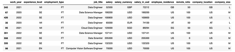
Below is the top 5 rows from the data set.

import pandas as pd

df = pd.read_csv('ds_salaries.csv', index_col = [0])

df.head()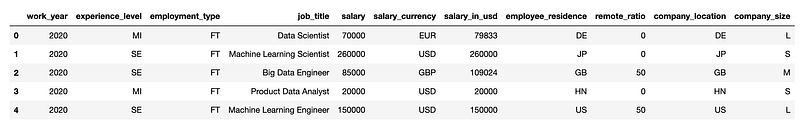

Pro Tip: When I ran the above, the entire width of the data frame did not fit in the view and I had to scroll left and right to see some of the columns. In order to fit everything in one view (so that I can paste it in one image here!), I used the lines below. Give it a shot!

from IPython.display import display, HTML
display(HTML("<style>.container { width:100% !important; }</style>"))

Now that we know more about the data set, let’s get started on the concepts and practice questions.

Tutorial + Questions and Answers

I will start with a brief overview of each concept and then most of the learning will be during the practice questions included for each topic. The Jupyter notebook including questions and answers is provided in the next section. To maximize learning, try to answer the questions yourself before looking at the notebook. Then look at the notebook to verify your answer.

1. Central Limit Theorem

Central Limit Theorem states that given a population with mean μ and standard deviation of 𝜎, when we collect sufficiently large random samples from that population (with replacement), then the distribution of the sample means will be approximately normally distributed, regardless of the population distribution. This concept is very powerful in practice because it allows us to assume a normal distribution for the sample means, which is a well known distribution for statistical analysis and inference.

Let’s look at this in practice to better understand it.

Question 1:

What is the average and standard deviation for the salary in our data set? Show the distribution of the salary, using a histogram and a box plot. Please use “salary_in_usd” for comparability purposes in all questions.

Answer:

Let’s first import all the libraries we will be using today.

import numpy as np
import pandas as pd
import matplotlib.pyplot as plt
import scipy.stats as stats
import math

%matplotlib inline

import warnings
warnings.filterwarnings('ignore')

Now let’s work on the answer.

# Method 1 - Using NumPy
print("Method 1 - Using NumPy")
print(f"Mean: {np.mean(df.salary_in_usd)}")
print(f"STD: {np.std(df.salary_in_usd)}\n")

# Method 2 - Using Pandas
print("Method 2 - Using Pandas")
print(f"Mean: {df.salary_in_usd.mean()}")
print(f"STD: {df.salary_in_usd.std()}")

Results:

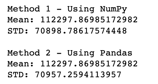
Let’s talk about the results.

First observation is how large the standard deviation is. That is something we can look into but since we want to focus on Central Limit Theorem, let’s skip that for now.

Second observation is that the standard deviations do not match between NumPy and Pandas. The reason behind the inconsistency is that Pandas uses n-1 in the denominator when calculating standard deviation, while NumPy does not do that by default (this has to do with the degrees of freedom considered in calculating the standard deviation). We can instruct NumPy to use the same, which results in the same standard deviation calculations, as demonstrated below.

Either one can be considered correct, depending on the use case and it is really not important for this exercise — this was provided in case you come across it in the future.

# Method 1 - Using NumPy
print("Method 1 - Using NumPy")
print(f"Mean: {np.mean(df.salary_in_usd)}")
print(f"STD: {np.std(df.salary_in_usd, ddof = 1)}\n")

# Method 2 - Using Pandas
print("Method 2 - Using Pandas")
print(f"Mean: {df.salary_in_usd.mean()}")
print(f"STD: {df.salary_in_usd.std()}")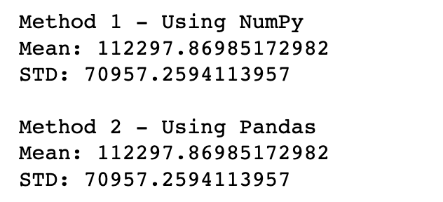

# Histogram of salary
plt.hist(df["salary_in_usd"], bins = 20)
plt.title("Histogram of Salaries")
plt.xlabel("Salary")
plt.ylabel("Frequency")
plt.show()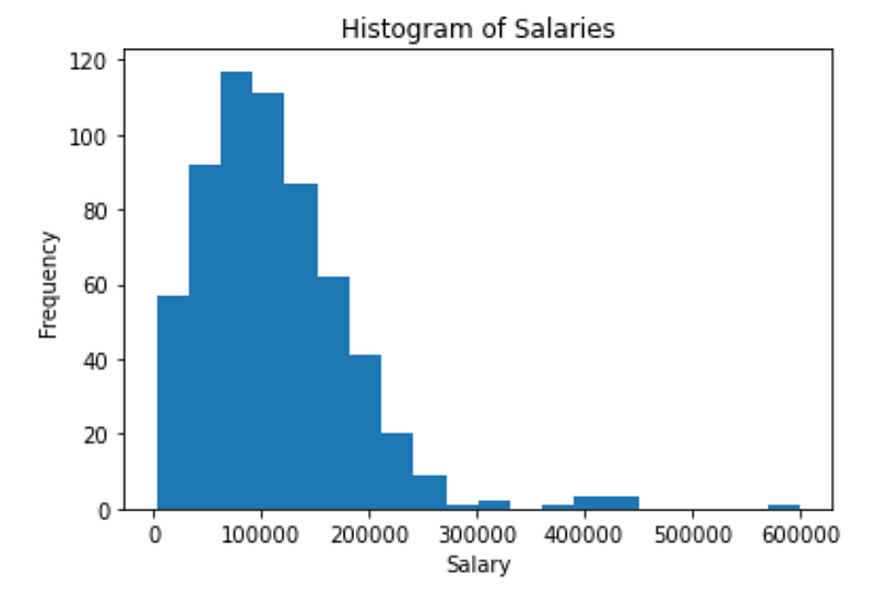

# Box plot of salary
plt.boxplot(df.salary_in_usd, vert = False)
plt.title("Box Plot of Salaries")
plt.xlabel("Salary")
plt.ylabel("Frequency")
plt.show()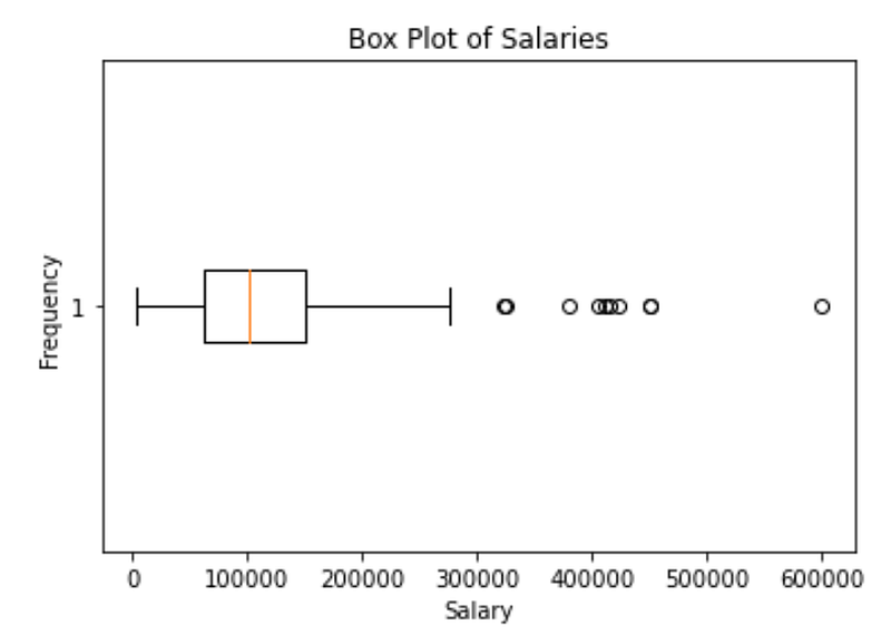

Since the goal of this exercise is to focus on Central Limit Theorem, we are not going to go deeper into the data to find out what is driving this right-skewed distribution but if you are curious, you can look at various slices of the data.

Question 2:

Now that you know the average of salaries in our data set (i.e. the population), verify the Central Limit Theorem using the following scenarios: 100 samples of size 10, which we will call 100 * 10, followed by 100 * 20, and 100 * 50. General steps to follow are:

1. Collect x * y samples with replacement from the population (i.e. salary). 2. Calculate the mean of the collected sample. 3. Create a histogram to visually verify the distribution of the mean of the collected samples

Hint: In order to collect samples, we can use: pandas.DataFrame.sample(n, replace = True.

Answer:

sample_sizes = [10, 20, 50]
bin_count = 25
total_samples = 100

for sample_size in sample_sizes:
    # An empty list to store means of collected samples
    list_of_sample_means = []
    
    for i in range(total_samples):
        sample = df["salary_in_usd"].sample(n = sample_size, replace = True)
        sample_mean = sample.mean()
        list_of_sample_means.append(sample_mean)
    
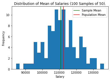
    plt.hist(list_of_sample_means, bins = bin_count)
    plt.title(f"Distribution of Mean of Salaries ({total_samples} Samples of {sample_size}).")
    plt.xlabel("Salary")
    plt.ylabel("Frequency")
    plt.axvline(x = np.mean(list_of_sample_means), label = 'Sample Mean', color = 'green')
    plt.axvline(x = df["salary_in_usd"].mean(), label = 'Population Mean', color = 'red')
    plt.legend(loc = "upper right")
    plt.show()

Results:

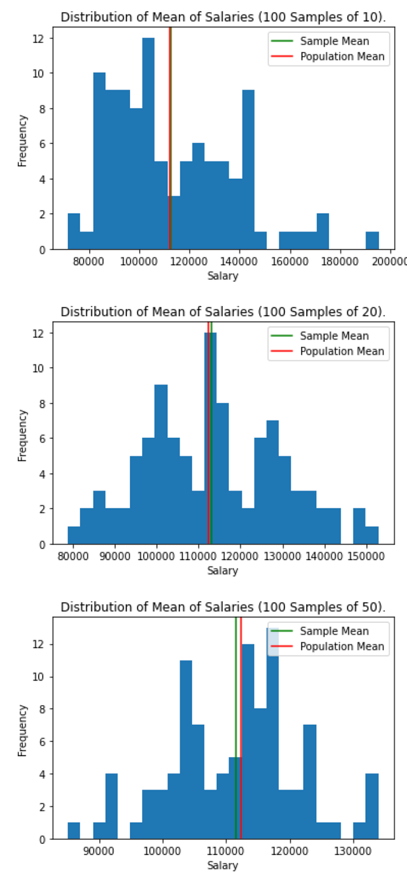
Takeaway: Comparing the results to the population distribution of “salary_in_usd”, we can see that as Central Limit Theorem stated, the distribution of the means of the collected samples are much closer to a normal distribution, although the distribution of the original population was further from normal.

2. Z-Score

Z-score tells us the distance of each point from the mean in terms of standard deviations. For example, Z-scores of 2 and -1 would indicate values are 2 standard deviations above and 1 standard deviation below the mean, respectively. Z-score is calculated as follows:

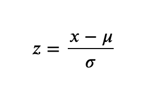
μ: Population Mean

𝜎: Population Standard Deviation

Question 3:

Sample a random salary from the data set, using “random_state = 1234” and calculate its Z-score.

Answer:

sample = np.array(df["salary_in_usd"].sample(n = 1, random_state = 1234))[0]
mu = df["salary_in_usd"].mean()
sd = df["salary_in_usd"].std()

z = (sample - mu) / sd

print(f"collected sample: {sample}")
print(f"population mean: {mu}")
print(f"population standard deviation: {sd}")
print(f"z-score: {z}")

Results:

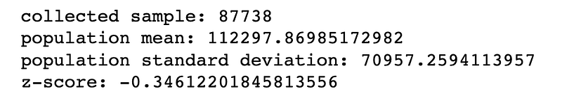
Z-score indicates that the collected sample is ~0.35 * standard deviation lower than the population mean.

3. Confidence Level and Confidence Interval

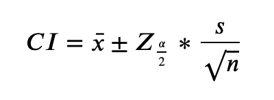
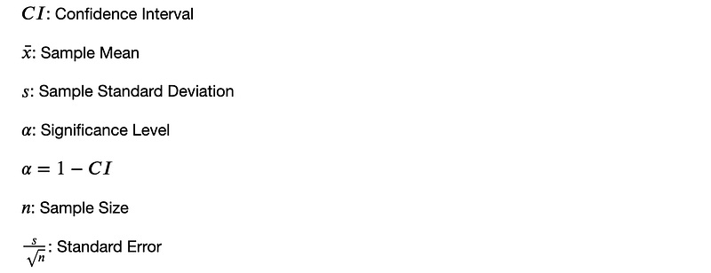
Let’s understand this concept with an example. If we generate all of the possible 95% confidence intervals (by sampling according to a 95% confidence level design), 95% of such intervals are expected to contain the parameter’s true value. This parameter is usually the population mean. As a result when we use a 95% confidence interval to collect many samples and through those samples estimate a population’s mean, there is a 95% chance that the confidence intervals include the population mean. Confidence interval or CI is calculated as follows:

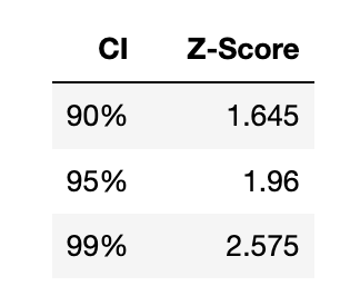
Z-scores can be calculated using a standard normal table and the most commonly used ones are as follows:

Question 4:

What is the Z-score for a confidence interval of 95%?

Answer:

print(f"Z-score for a 95% confidence interval is {stats.norm.interval(0.95)}")

Results:

Question 5:

Collect 100 samples of the salaries and calculate the upper and lower bounds of a 95% confidence interval around the sample mean.

Answer:

ci = 0.95
n = 100
# collect the sample
sample = df["salary_in_usd"].sample(n = n, replace = True)
# calculate sample mean
x = np.mean(sample)
# calculate sample standard deviation
sd = np.std(sample, ddof = 1)
# calculate z-score
z = stats.norm.interval(ci)[1]
# calculate upper and lower bounds of the confidence interval
ub = x + z * sd / math.sqrt(n)
lb = x - z * sd / math.sqrt(n)
print(f"95% confidence interval extends from {lb} to {ub}.")

Results:

Question 6:

Based on the definition of a 95% confidence interval, we expect the population mean to be within the calculated confidence interval at 95% of the times. Validate this by collecting 100, 1000, 10000, and 100000 samples of 100.

Pro Tip: This question might seem a bit daunting at first, if you are newer to writing Python function, I have two suggestions: (1) What I usually find helpful is to forget about writing a function or even a loop and just try to write the code that does one round of sampling and then calculates the confidence interval. Then make it a bit more advanced and add a loop that can repeat the same process for different samples mentioned in the question. Finally, make it a function. (2) If you feel that you need more practice on Python Functions you can work through more Python Functions practice questions in my post here.

Answer:

def probability_calculator(ci=0.95, n=100, ct=1000):
    population_mean = np.mean(df.salary_in_usd)
    counter = 0

for i in range(ct):
        # collect the sample
        sample = df["salary_in_usd"].sample(n = n)
        # calculate sample mean
        x = np.mean(sample)
        # calculate sample standard deviation
        sd = np.std(sample, ddof = 1)
        # calculate z-score
        z = stats.norm.interval(ci)[1]
        # calculate upper and lower bounds of the confidence interval
        ub = x + z * sd / math.sqrt(n)
        lb = x - z * sd / math.sqrt(n)
        if (population_mean < ub) and population_mean > lb:
            counter += 1
            
    print(f"In {round(counter/ct, 4)*100}% of {ct} collected samples, population mean was inside the calculated 95% confidence interval.")
    
repeat_list = [100, 1000, 10000, 100000]

for repeat in repeat_list:
    probability_calculator(ci, n, ct = repeat)

Results:

As expected, at around 95% of instances, population mean lies inside the confidence interval.

4. Sample Size Calculation

In the previous sections, we learned how to calculate the Z-score and a confidence interval. Now we are going to look into the minimum sample size required to achieve a desired confidence level. For this purpose, we can re-arrange the Z-score formula as follows:

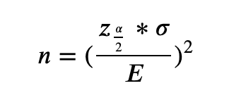
n: Minimum Sample Size

𝜎: Population Standard Deviation

E: Accepted Level of Error

Let’s use this in an example to better understand it.

Question 7:

How many samples do we need to collect from our salary data for a 95% confidence level with an accepted error of $10,000?

Answer:

cl = 0.95
sd = np.std(df.salary_in_usd)
z = stats.norm.interval(cl)[1]
e = 10000
n = (z * sd / e) ** 2
print(f"Minimum sample size at {cl} confidence level: {round(n, 0)}")

Results:

Question 8:

How would the minimum sample size change if we wanted a 90% confidence interval (all else similar to Question 7)? Before solving the problem, think through whether we should expect the minimum sample size to increase or decrease.

Answer:

Since the confidence level required is lower, we expect the minimum sample size required to achieve this confidence level to also be lower, compared to the previous question. Let’s verify using actual data.

cl = 0.9
sd = np.std(df.salary_in_usd)
z = stats.norm.interval(cl)[1]
e = 10000
n = (z * sd / e) ** 2
print(f"Minimum sample size at {cl} confidence level: {round(n, 0)}")

Results:

5. Sampling Strategies

We are going to look into two of the most common sampling strategies, as follows: - Simple Random Sampling - Stratified Random Sampling

5.1. Simple Random Sampling

Simple Random Sampling is when we randomly select the data points from a population. This might not always be the best way to collect samples but it is one of the easiest ways.

Let’s see how this is done in Python.

Question 9:

Collect 9 random samples from our original data set.

Answer:

df.sample(n = 9, replace = False)

Results:

As we can see, 9 rows of the original data frame are randomly selected and returned here.

Now let’s look at other sampling strategies.

5.2. Stratified Random Sampling

Stratified Random Sampling (or Stratified Sampling) is when samples are collected based on the proportions existing in the population. For example, if the population includes two groups of A, representing 80% of the data and B, representing the remaining 20% of the data, then in a stratified sampling approach we will collect 80% of the samples from A and the remaining 20% from B.

Let’s look at an example.

Question 10:

If we were to implement a stratified sampling strategy to make inferences about the salaries, determine the percentage of samples that should be collected from each company size group.

Then calculate minimum sample size required for a 95% confidence level with an accepted error of $10,000 for each of those groups.

Answer:

First, let’s group salaries by company size:

# Group by company size
sample_weight = df[['salary_in_usd', 'company_size']].groupby('company_size').count().sort_values('company_size', ascending = False)
sample_weight['sample_weight'] = sample_weight['salary_in_usd'] / sample_weight['salary_in_usd'].sum()
sample_weight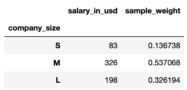

As we can see in the results, the weights are different for each company size and total of the sample weights equals 1, which is as expected.

Next, we will calculate the minimum sample size required based on the desired confidence level.

# Calculate minimum sample size required
cl = 0.95
sd = np.std(df.salary_in_usd)
z = stats.norm.interval(cl)[1]
e = 10000
n = (z * sd / e) ** 2
print(f"Minimum sample size at {cl} confidence level: {round(n, 0)}")

Now that we know how many samples are required, we calculate sample size per stratum (i.e. group):

# Calculate minimum sample size for each group
sample_weight ['sample_size'] = round(sample_weight['sample_weight'] * n, 0)
sample_weight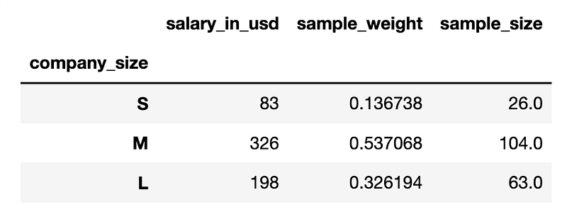

As we see in the results, the sample sizes are determined based on the original weight of each of those strata (i.e. S, M and L) in the population.

Notebook with Practice Questions

Below is the notebook with both questions and answers that you can download and practice.

Thanks for Reading!

If you found this post helpful, please follow me on Medium and subscribe to receive my latest posts!