10 Best Beginner Friendly Pandas Function to kickstart your Data Science Journey

Introduction

Python has become one of the or THE language when it comes to Data Science projects. With the advent of Jupyter Notebooks and Jupyter Lab. It has become effortless to spin up simple Machine learning Models or run statistical analysis on the data that you have.

For python packages Pandas is the best library for data manipulation and analyses. This provides you with the necessary tools that you can leverage to start layering the foundation for these data science projects. In this post, I will be going through the most useful pandas functions that I use time and again when I am working on said such projects.

Pandas is a Python package providing fast, flexible, and expressive data structures designed to make working with “relational” or “labeled” data both easy and intuitive.

You have multiple columnar data and you want to understand the relationships between the columns and rows. Pandas help you derive insights by making it easier to understand.

I have taken the Video Game Sales Dataset available in Kaggle to illustrate the applications of these functions.

Before running these functions make sure to install the necessary library and imports.

!pip install pandas
import pandas as pd

Algorith Series: I recently did a 100 Days to Amazon Challenge you can start from Day 1.

1) Read_csv()

This function is used for reading the data that is stored in Comma-Separated Values (CSV) is a file format and load it as a data frame. With which you can manipulate the data in more transparent and nimble fashion. You have to specify the location of the csv file as a parameter to retrieve the data.

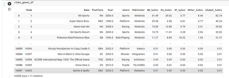
video_games_df = pd.read_csv(‘/content/sample_data/vgsales.csv’)

The dataframe will look like:

2) Describe()

Now you have taken a look at the data but you don’t know what you can infer from this. Describe function gives you the standard aggregate functions such as the count, min, max, mean and standard deviation for each column of the data frame. With this you can gain a quick insight of the data that you have and represent it with numbers.

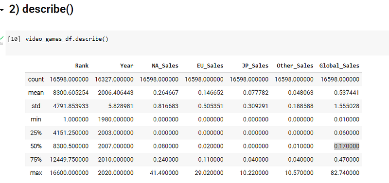
You can see Rank has 16598 values and only 163237 year values which means there are null values in the rows for year. We can instantly now from this that we have to handle null values in this dataset.

This library gives you a general understanding of the dataset what if you wanted to know about the specific unique data that data has?

3) Nunique()

This function returns the number of distinct / unique elements present in each column of the dataframe.

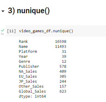
You only knew there were around 17000 Ranked sales record. But now from this, we have data that span 39 years. With 12 Known Genres (sports, action, .. ) and across 31 Platforms(PS2, Xbox, PS4) and 500+ publishers.

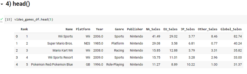
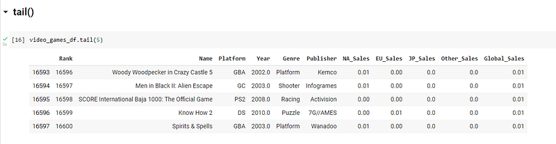
4) Head() and Tail()

Now you have loaded the dataset into the dataframe. You want to take a quick peek at the data before even starting to comprehend it and derive insights from the data. For this you can swiftly use the said functions to take a look at the start or bottom of the dataset and understand what the data holds.

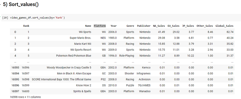
5) Sort_values()

As the name suggests this function allows you to sort the rows of the dataframe based on the values of a specific column or a list of columns. You can specify the order in which the data has to be sorted ascending or descending.

Note : You do not have two different parameters for the sorting order. You have to specify ascending ==False. So that the data is sorted in descending order.

I will explain how the multiple column sorting works. In essence, you will be sorting multiple times based on the result of the previous sorts. Take a look at the following

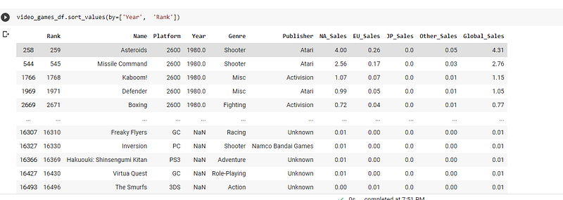
Here the dataframe is sorted by the year and then in each year which of the games have placed the highest rank. This is a great way to derive multiple combinations of insights.

• In every year which record had more sales?
• In every year which Platform had the most sales?

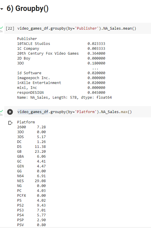
6) GroupBy()

This function allows you to gain a quick insight of the common aggregate functions based on user defined columns. Let’s say you want to know the mean/median/average sales of each publisher across North America. You can structure it with the help of this function.

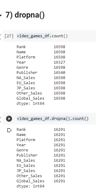
7) Dropna()

This function aids in preprocessing your dataset to handle null value rows which might introduce noise.

• This function drops the row with any/all null values present in it’s columns. This condition can be set with the help of ‘how ’parameter in the function.
• If you want to drop a row if all it’s values are null then use how = “all”, if you want to drop a row if any of the column value is null use how = “any”..

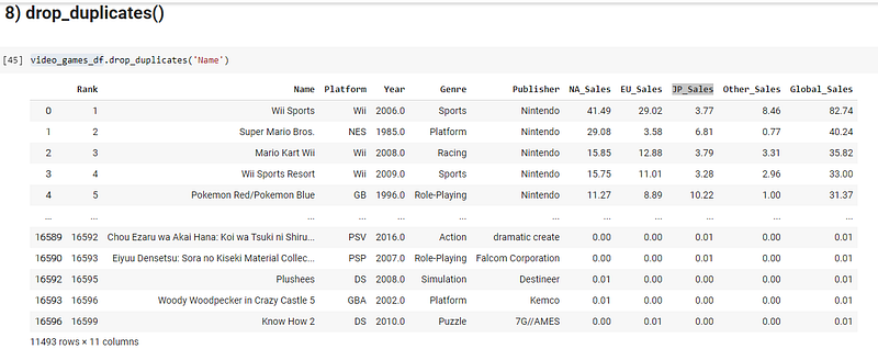
8) Drop_duplicates()

Usually the raw dataset that we have comes with a lot of noise values, like null values, repeated values and anomalies. You just saw how to handle null values. A model trained on repeated values or duplicates will be lenient towards the duplicated rows.

9) Apply()

Now, let’s say if you want to change the entire value of a column based on your need. One way of solving it is to iterate through each row and change the required value. The simplest example would be changing the unit of a specific column like (C-F, lbs-kg, m-km)

Instead of iterating, you can use a lambda function and apply that function on each row in a single line of code.

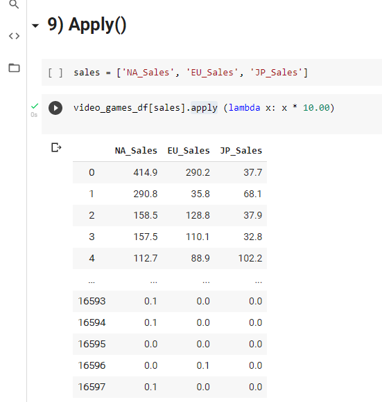
Not only can you change a specific column, you can change multiple columns parallelly.

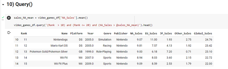
10) Query()

As the name suggests, this can be used to run a specific query on your dataframe and return the results as a Dataframe. You can include different variables into the query by adding @ before the variable inside the query statement.

End of the Line

Thank you for reading the Article. Next post coming soon!

Don’t forget to hit the follow button✅ to receive updates when we post new coding challenges. Tell us how you solved this problem. 🔥 We would be thrilled to read them. ❤ We can feature your method in one of the blog posts.