
N-BEATS — The First Interpretable Deep Learning Model That Worked for Time Series Forecasting
An easy-to-understand deep dive into how N-BEATS works and how you can use it.
Time series forecasting has been the only area in which Deep Learning and Transformers did not outperform other models.
Looking at the Makridakis M-competition, the winning solutions always relied on statistical models. Until the M4 competition, winning solutions were either pure statistical or a hybrid of ML and statistical models. Pure ML approaches barely surpassed the competition baseline.
This changed with a paper published by Oreshkin, et al. in 2020. The authors published N-BEATS, a promising pure Deep Learning approach. The model beat the winning solution of the M4 competition. It was the first pure Deep Learning approach that outperformed well-established statistical approaches.
N-BEATS stands for Neural Basis Expansion Analysis for Interpretable Time Series.
In this article, I will go through the architecture behind N-BEATS. But do not be afraid, the deep dive will be easy-to-understand. I also show you how we can make the deep learning approach interpretable. However, it is not enough to only understand how N-BEATS works. Thus, I will show you how we can easily implement a N-BEATS model in Python and also tune its hyperparameters.
Let’s understand the core idea of N-BEATS before looking at its architecture.
The core functionality of N-BEATS lies in neural basis expansion.
Basis expansion is a method to augment data. We expand our feature set to be able to model non-linear relationships. Sounds abstract, right?
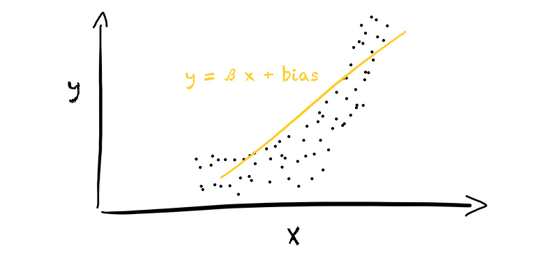
How does basis expansion work? For example, we have a problem in which our target value y stands in some relationship to a feature x. We want to represent the relationship between y and x using a linear model. In the 1d space, this will result in a linear relationship (left plot in the figure below).
However, the feature and target might not show a linear relationship, resulting in a useless model. Is there anything we can do?
Yes, we can expand our feature set. Let’s add the quadratic value of the original feature to the feature set, resulting in [x, x²]. With this, we moved from a 1d space into a 2d space since we now have two features instead of one. We can now fit a linear model in the 2d space, resulting in a second-degree polynomial model (right plot in the figure below).
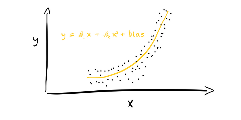
And this is all there is to basis expansion. We extend our feature set by adding new features based on the original features. In this case, we used a polynomial expansion of degree 2. We added the quadratic value of each original feature to the feature set.
The most common basis expansion method is polynomial basis expansion. Yet, there are many other approaches, such as binning, piecewise-linear splines, natural cubic splines, logarithms, or squares.
The N-BEATS model decides which basis expansion to use. During training, the model tries to find the best basis expansion method to fit the data. We let the model do the work. That is why it is called ”neural basis expansion.”
How does N-BEATS work in detail?
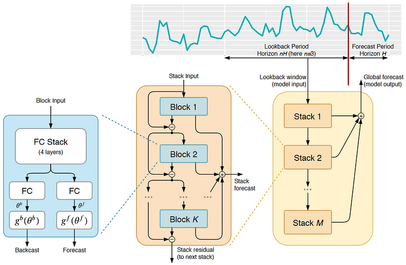
The N-BEATS model has the following architecture:
A lot is going on here, and the picture might be overwhelming. But, the idea behind N-BEATS is straightforward.
We can observe two things.
First, the model splits the time series into a lookback and forecast period. The model uses the lookback period to make a forecast. The lookback period has multiple lengths of the forecast period. An optimal multiple usually lies between two and six.
Second, the N-BEATS model (yellow rectangle on the right) consists of layered stacks. Each stack, in turn, consists of layered blocks.
Each block has a fork-like structure (blue rectangle on the left). One branch in the block produces a backcast, and the other branch a forecast from some block input data. The forecast contains the prediction of unseen values. The backcast, in contrast, shows us the model’s fit on the input data.
How do we receive the backcast and forecast from the input? First, the model passes the input through a fully connected neural network with four layers. The MLP produces the expansion coefficients, theta, for the backcast and forecast. These expansion coefficients flow into two branches, one for backcasting and one for forecasting. In each branch, we perform the basis expansion. Here, the actual “neural basis expansion” happens.
As we can see in the picture above, N-BEATS connects various blocks in a stack. Because each block returns a backcast and forecast, two things happen. First, the model adds the partial forecast of each block to produce the stack’s forecast. Second, the model removes the backcast of a block from the block’s input. Hence, each block only receives the residual of the previous block. With this, the model only passes information that is not captured by the previous block to the next. Hence, each block tries to approximate only a part of the input signal, focusing on local patterns.
The N-BEATS model then layers various stacks. Like the blocks in a stack, each stack, except the first one, is trained on the residuals of the previous stack. With this, each stack learns a global pattern that was not captured before. The final forecast is the sum of the stack’s forecasts, providing a hierarchical decomposition.
As we can see, N-BEATS applies a double residual stacking approach. The backcast and forecast result in backward and forward residuals. The layered architecture of blocks and stacks leads to the stacking of these residuals. Through the double residual stacks, N-BEATS can recreate the mechanisms of statistical models.
The advantages of N-BEATS
Compared to other deep learning approaches, N-BEATS enables us to build very deep NNs with interpretable results. Moreover, the training is faster. The model does not contain any recurrent or self-attention layer. Its double residual stacking facilitates a more fluid gradient backpropagation.
Compared to classical time series forecasting approaches, we do not need to do any feature engineering. We do not need to identify time series-specific characteristics, like seasonality and trend. N-BEATS does this for us. This makes the model easy to use, and we can get quickly started.
Moreover, the model is capable of Zero-Shot Transfer Learning.
How can the deep learning architecture be interpretable?
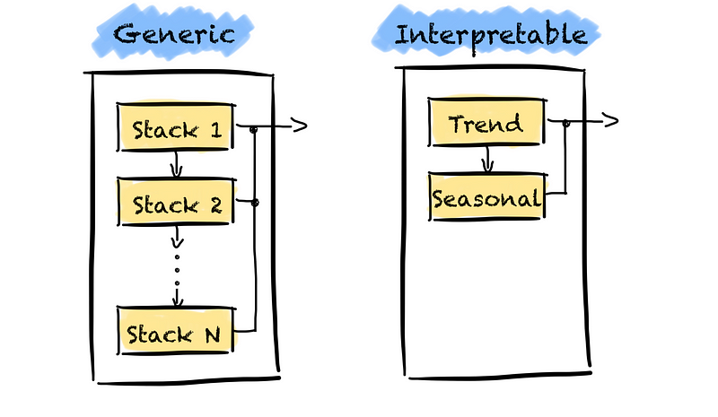
Well, the generic version of N-BEATS, I described above, is not interpretable. There are no constraints on what basis functions the model can learn and the depth of the network. We do not know what the model learns and if these are time series-specific components, such as trend.
How do we gain interpretability?
There apply a trick. We restrict the depth of the model and which basis expansion functions the model can learn.
For example, we often use trend and seasonality in time series forecasting.
We can force the model to learn only these two characteristics. First, we restrict the depth of the model by only using two stacks. The first stack learns the trend, and the second stack learns the seasonality.
We can then interpret the model’s results by extracting each stack’s partial forecasts.
Second, we must force the model to learn the trend and seasonality only. We must introduce a problem-specific inductive bias. We achieve this by setting the basis expansion functions to specific functional forms. For this, we replace the last layer in each block with a function. We use a polynomial basis to determine the trend and a Fourier basis for seasonality.
Forecasting example using N-BEATS
Now that we know how N-BEATS works, let’s apply the model to a forecasting task.
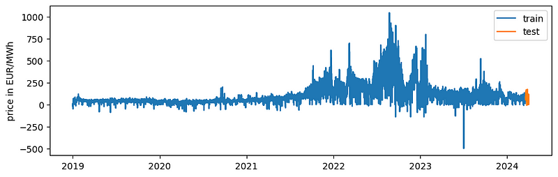
We will predict the next two weeks of wholesale electricity prices in Germany. The data is provided by Ember in the “European Wholesale Electricity Price” under a CC-BY-4.0 license. We will use the N-BEATS implementation from Nixtla’s neuralforecast library. The library makes it very easy for us to apply N-BEATS.
Please note that I am not trying to get a forecast as accurate as possible but rather show how we can apply N-BEATS.
Alright. Let’s get started.
Let’s import all the libraries we need and the dataset.
Nixtla has a time series format that every model expects. The time series format is a DataFrame with columns ds containing the timestamps, y containing the target value, and unique_id which is a unique identifier. The unique_id allows us to train a model on different time series simultaneously.
We will skip a detailed data exploration step here. However, we can see two seasonal components:
- daily: Prices are higher in the morning and evening hours as the electricity consumption is usually higher during these hours.
- weekly: Prices are higher on weekdays than on weekends as electricity consumption is usually higher during weekdays.
The next step is splitting our dataset into a training and test set. As I want to forecast the next two weeks of consumption, I use the last two weeks of the dataset as my test set.
I had some trouble getting the model to work when using Panda’s Datetime. Hence, I converted the date time into timestamps.
Finally, I created a function to plot the results.
Baseline Model
For completeness, we will start with a simple model as our baseline. I have written about baseline models and why you should start with them in another article.
We will use a seasonal naïve baseline model as the consumption shows different seasonality patterns. We will use the SeasonalNaive model provided in Nixtla’s statsforecast library. Here, we take the last week of data in the training set as our forecast.
The results look quite good. The baseline gives us a MAE of 17.84. The accuracy of the baseline is very good in the first week of the test set. However, the further we are away from the last known value, the smaller the accuracy.
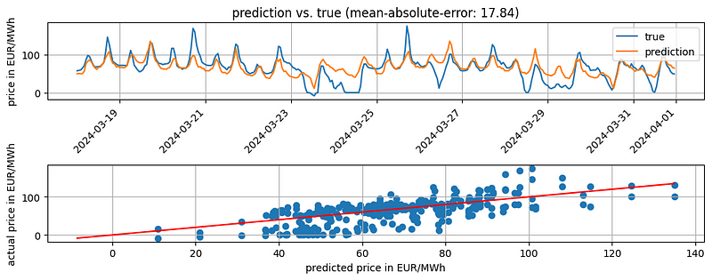
We probably could do better if we spend more time on the baseline model. However, the baseline should be good enough for our use case.
Training the N-BEATS model
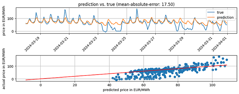
Let’s train our first N-BEATS model. The implementation is straightforward. We initialize our N-BEATS model, defining our forecast and lookback period. In this case, I use a lookback period of two week.
Then, we have some customization options. We can customize
- the model by choosing stack types, number of blocks, size of the MLP layers, activation function, etc.
- the training by choosing the loss function, learning rate, batch size, etc.
- the scaling of our input data.
See the Nixtla’s documentation for a full description. In the code snippet, I have already played around with the hyperparameters.
Once we have initialized our model, we must wrap it with the neuralforecast class. The class provides us with methods we need to train the model and later make predictions. Also, the class allows us to train different models by passing a list of models to models.
Then, we can finally fit the model using the fit() method and run a prediction for the next month.
The results look slightly better than our baseline. The MAE goes down to 17.5 compared to 17.84 of our baseline.
Tuning the hyperparameters of the N-BEATS model
Instead of playing around to find good hyperparameters, let’s run a hyperparameter optimization.
It is not complicated. Nixtla provides us with an AutoNBEATS model, doing the hyperparameter tuning. We can choose between ray and optuna as the backend and either use a default config for the hyperparameters or create a custom config. We define our choices when initializing the AutoNBEATS model. That is the only difference compared to running the NBEATS model. All other steps stay the same.
In this case, I will use Optuna and a custom config file.
Running the predict() method after the hyperparameter tuning gives us predictions using the best model.
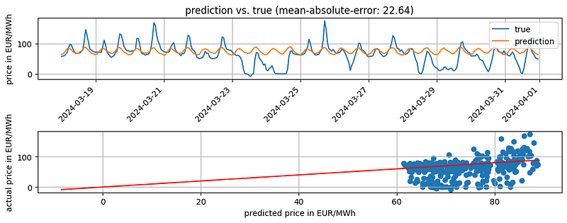
We see that the “optimized” N-BEATS has a worse accuracy (MAE of 22.64) compared to the baseline and N-BEATS model. However, running more trials during the hyperparameter tuning with a different search space might result in different results.
If we do not pass a config to the model, AutoNBEATS uses the default config. If we only want to change a few parameters from the default config, we could run this snippet.
If you want to see the results of the hyperparameter tuning, you can get them from the results attribute of the model.
# show results of hyperparameter tuning runs
results = fcst.models[0].results.trials_dataframe()
N-BEATS with exogenous variables
Before I finish this article, I want to show you one last thing. We can also use exogenous variables in the N-BEATS model. For this, we only need to use Nixtla’s NBEATSx and define what exogenous variables we want to use. For example, we could pass the hour of the day to the model as there is a daily seasonality.
Adding the day of the week as an exogenous variable resulted in a MAE of 19.58. However, trying different exogenous variables, such as electricity consumption or generation forecast, or different hyperparameters could improve the accuracy.

A final note on the examples
In all the examples, I showed you a very static approach. We only make a forecast once on the test set. But let’s say we work for a company that owns some power generation units. The company wants to know how they should plan the operation of their units to maximize revenue. For this, they want an updated forecast every morning. Hence, we must run the model every day.
But how do we manage? Above, we only predicted the weeks directly after the training set.
We always need to re-train our model when we want to make a new prediction. The N-BEATS model relies on the lookback period. Hence, we must update our data set with the latest available data and train the model again. In our example, the wholesale price of the last day.
Should we run our hyperparameter tuning as well? Probably not. The tuning can take quite a long time and be computationally expensive. Instead, we run the hyperparameter tuning on the train set once. We use the same hyperparameters when re-training the model every day. If we see that the model degrades too much over time, we can re-run the hyperparameter tuning.
Conclusion
The article has been very long. Longer than I intended. But there was a lot to cover. If you stayed until here, you now should
- have a very good understanding of how the N-BEATS model works
- be able to use the N-BEATS model in practice and
- be able to change the model’s inner workings during your hyperparameter tuning.
If you want to dive deeper into the N-BEATS model, check out the N-BEATS paper. Otherwise, leave a comment and/or see you in my next article.


